31
QUEEN MARY UNIVERSITY OF LONDON Simulation of the dynamics of a 2D fluttering aerofoil with a trailing edge flap DEN410 Aeroelasticity Reena Thapa Student Id:-090242902 14 th April 2014
| Date post: | 14-Jan-2017 |
| Category: |
Engineering |
| Upload: | sagar-chawla |
| View: | 37 times |
| Download: | 0 times |
Queen Mary University of London
Simulation of the dynamics of a 2D fluttering aerofoil with a trailing edge flap
DEN410 Aeroelasticity
Reena ThapaStudent Id:-090242902
14th April 2014
Abstract
Understanding the deformation due to aerodynamics forces is vital when designing an aircraft, especially on the aircraft wing. This report explores the wing divergence and bending-torsion flutter based on computer aided simulations. As a simulation tool, MATLAB has been used to simulate the two-dimensional aerofoil model with the trailing edge flap. Three set of simulations, out of which two were carried out for the two degree of freedom model with and without C(k) and the third simulation was carried out for three degree of freedom model that included the trailing edge flap. It was found that the flutter was avoided for the simulation without C(k) as U/b increases. However, the case was not similar for the simulation with C(k) as some flutter were present. Finally for the three degree of model simulation, flutter was present throughout the system.
Table of ContentsAbstract......................................................................................................................................1
1.Introduction.............................................................................................................................2
1.1 Aims and Objectives........................................................................................................2
2. Background Theory................................................................................................................2
3.Simulation Procedure..............................................................................................................9
4. Results..................................................................................................................................13
4.1 The Simulation results of two degree of freedom aerofoil model without C(k)...........13
4.2 The Simulation results of two degree aerofoil model with C(k)....................................15
4.3 The Simulation results of three degree of freedom aerofoil with flap...........................17
5. Discussion............................................................................................................................22
6. Conclusion............................................................................................................................23
7. References............................................................................................................................23
Reena Thapa Page 1
1.IntroductionAeroelasticity explores the interaction of inertial, structural and aerodynamic forces on aircraft, building or any other surfaces. Aeroelastic problems would not exist if airplane structures where perfectly rigid. Modern airplane structures are very flexible, and this flexibility is fundamentally responsible for the various types of aeroelastic phenomena (Bisplinghoff,1996). Flutter is a dangerous phenomena that is encountered in aircraft wings. In an aircraft, as the speed of the wind increases, there may be a point at which the structural damping is insufficient to damp out the motions which are increasing due to aerodynamic energy being added to the structure. This vibration can cause structural failure and therefore considering flutter characteristics is an essential part of designing an aircraft.
In aircraft wings, flutter may indeed become problematic due to the flap control. It is thus important to predict the effects of the trailing edge control systems on the stability limits (Bergami, 2008). Therefore, Stability is analysed through an aeroelastic investigation of a representative 2D aerofoil section equipped with a trailing edge flap.
1.1 Aims and ObjectivesThe aim of the simulation is to investigate the factors governing the response of a three degree of freedom aerofoil model with a trailing edge flap, in relation to basic analytical techniques. In order to achieve this aim, the following objectives were implemented:
Familiarisation with basic dynamics and control of a two-dimensional aerofoil with a trailing edge flap.
Implement the simulation tool called MATLAB to simulate the dynamics of a two-degree of freedom and three-degree of freedom aerofoil model, both with trailing edge flap.
Assessment of the design of the controller and performance features. Understand the dynamics with reference to an aeroelastic system. Employ the simulation to predict the flow speed at which flap equipped system
may become unstable due to static and dynamic instabilities i.e. wing divergence and bending-torsion flutter.
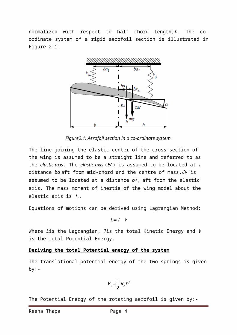
2. Background TheoryIn this investigation, the aerofoil section is modelled as a rigid flat plate which has a mass, m. The aerofoil section do not deform but it moves in the plane. The three degree of freedom is described by the torsion or pitch rotation of the aerofoil as the angle α between the aerofoil chord and the x axis. . The wing stiffness is idealized and represented by two springs K A and K B. The chord of the wing is assumed to be 2 b . The origin of the co-ordinate system is assumed to be located at the elastic centre of the cross-section which is assumed to be located at EA. The co-ordinates on the system are given in dimensionless form, distances from the
Reena Thapa Page 2
origin are in fact normalized with respect to half chord length,b. The co-ordinate system of a rigid aerofoil section is illustrated in Figure 2.1.
Figure2.1: Aerofoil section in a co-ordinate system.
The line joining the elastic center of the cross section of the wing is assumed to be a straight line and referred to as the elastic axis. The elastic axis (EA) is assumed to be located at a distance ba aft from mid-chord and the centre of mass,CM is assumed to be located at a distance bxα aft from the elastic axis. The mass moment of inertia of the wing model about the elastic axis is I α.
Equations of motions can be derived using Lagrangian Method:
L=T−V
Where Lis the Lagrangian, T is the total Kinetic Energy and V is the total Potential Energy.
Deriving the total Potential energy of the system
The translational potential energy of the two springs is given by:-
V 1=12
k hh2
The Potential Energy of the rotating aerofoil is given by:-
V 1=12
k α α 2
The Potential Energy of the trailing edge flap while rotation is given by:-
V 3=12
kβ β2
Therefore the total potential energy of the aerofoil section including the trailing edge flap is:
Reena Thapa Page 3
V=V 1+V 1+V 3
V=12(kh h2+b2kα α 2+kβ β2)
Deriving the total Kinetic energy of the system
The translational vertical motion of the wing with the trailing edge flap included, gives the Kinetic Energy at the centre of mass:
T 1=12
m(h+b xα α )2
A rotational component of the Kinetic Energy due to rotation of the aerofoil can be expressed as:
T 2=12
ICM α2
Where ICM = Mass moment of inertia
According to the parallel axis theorem the mass moment of inertia about the centre of mass is related to the mass moment of inertia about the elastic axis. Their relation is defined as:
I CM=( I α−m (b xα )2 )
The total kinetic energy of the system is also affected by the trailing edge flap. Measured from the centre of gravity of the flap, the vertical displacement of the trailing edge flap is given as:
hβ=h+α ( c−a+xb ) b
The trailing edge flap is deflected by bx β β .
The Total Kinetic Energy of the trailing edge flap due to the vertical displacement can be expressed as:
T 3=12
mβ [( hβ+b xβ β )2− hβ2 ]
Therefore, the total Kinetic Energy of the aerofoil and the flap together is given by:
T=12
m(h+b xα α )2+12
I CM α 2+ 12
mβ[ (hβ+b x β β )2−hβ2 ]
The equations of motion can be obtained by inserting the expressions for the total energy into Langrange’s equation.
Reena Thapa Page 4
ddt ( ∂ T
∂ q )−∂ L∂q
=0
ddt
∂ [[ 12
m (h+b xα α )2+ 12
I CM α 2+ 12
mβ [( hβ+b xβ β )2−hβ2 ]]+[ 1
2k hh2+ 1
2k α α 2+ 1
2kβ β2]]
∂ h−
∂[ [[12
m (h+b xα α )2+ 12
I CM α 2+ 12
mβ [( hβ+b xβ β )2−hβ2 ]]]+[1
2khh2+ 1
2b
2
k α α 2+ 12
b2
kβ β2]]∂ h
=0
This should yield a set of two equations of the form:
m h+mb xα α+kh h=0
mb xα h+ I α α+k α α=0
Given that the aerodynamic restoring force and restoring moment about the elastic axis, are L and M respectively, the disturbance force and moment are LG and M G, show that the equations of motion in inertia coupled form are:-
m h+mb xα α+kh h+L=LG
And
mb xα h+ I α α+k α α +M=M G
Generally, the restoring lift and moment may be only expressed as convolution integrals.
However, by making certain constraining assumptions that the motion is purely simple
harmonic, it can be shown that:
[ LM ]=M a[ h
α ]+Ca[ hα ]+ Ka[hα ]
Where
M a=πρ b3[ 1b
−a
−a b(a2+ 18 )]
Ca=πρ b3U [ 2 C (k )b
1+C (k ) (1−2a )
−C (k ) (1+2a ) b ( 12−a)( 1−C (k ) (1+2 a ) )]
K a=πρb U 2 C (k )[0 20 −b (1+2 a )]
Reena Thapa Page 5
Where C(k) is a complex function (the so called Theodorsen function) of the non-dimensional
parameter, k=ωb /U , (known as the reduced velocity) and U is the velocity of the airflow
relative to the aerofoil. As the aerodynamic stiffness matrix alone is a function of the square
of the velocityU2, one may ignore the effects of aerodynamic inertia and damping in the first
instance.
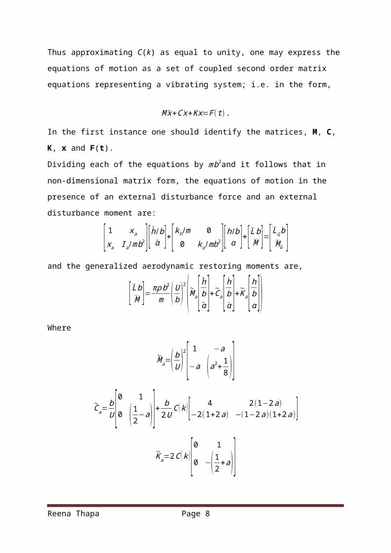
Thus approximating C(k) as equal to unity, one may express the equations of motion as a set
of coupled second order matrix equations representing a vibrating system; i.e. in the form,
M x+C x+Kx=F (t) .
In the first instance one should identify the matrices, M, C, K, x and F(t).
Dividing each of the equations by m b2and it follows that in non-dimensional matrix form, the
equations of motion in the presence of an external disturbance force and an external
disturbance moment are:
[ 1 xa
xa I a/mb2] [ h/bα ]+[kh/m 0
0 kα /mb2] [h/bα ]+[Lb
M ]=[LG bM G
]and the generalized aerodynamic restoring moments are,
[LbM ]= πρb2
m ( Ub )
2(~M a [ hbα ]+~Ca[ h
bα ]+~Ka[ h
bα ])
Where
~M a=( bU )
2[ 1 −a
−a (a2+ 18 )]
~Ca=bU [0 1
0 ( 12−a)]+ b
2 UC (k )[ 4 2(1−2a)
−2(1+2 a) −(1−2 a)(1+2a)]~Ka=2C ( k )[0 1
0 −( 12+a)]
And,LG and M G are an external non-dimensional disturbance vertical force and an external
disturbance anti-clockwise moment due to a typical gust. The equations of motion of the
aerofoil including the trailing edge flap may be expressed as:
Reena Thapa Page 6
[ mb2 m b2 xα mβ b2 x β
mb2 xα I α m β b2 x β (c−a )+ I β
mβ b2 xβ mβ b2 x β (c−a )+ I β I β][ h
bαβ ]+[khb2 0 0
0 k α 00 0 k β
][ hbαβ ][ Lb
−M−M β
]=[000]The last vector on the left hand side of above equation represents the generalised aerodynamic restoring moments.The generalised aerodynamic restoring moments can be expressed as:
[ Lb−M−M β
]=πρ b3U 2(~M a[ hbαβ ]+~Ca[ h
bαβ ]+~Ka[ h
bαβ ])
Where
~M a=( bU )
2[ 1 −aT 1
π
−a (a2+18 ) 2
T13
πT1
π2
T 13
π−T 3
π 2] ,~C a=
~C anc+~Cac−ntl+
~Cac−tl C (k ) ,
~Canc=bU [ 0 1
−T 4
π
−1 0T 15
πT 4
π−T 15
π0 ] ,~Cac−ntl=
bU [ 0
1−T 4
π ] [1(12−a) T 11
2 π ]
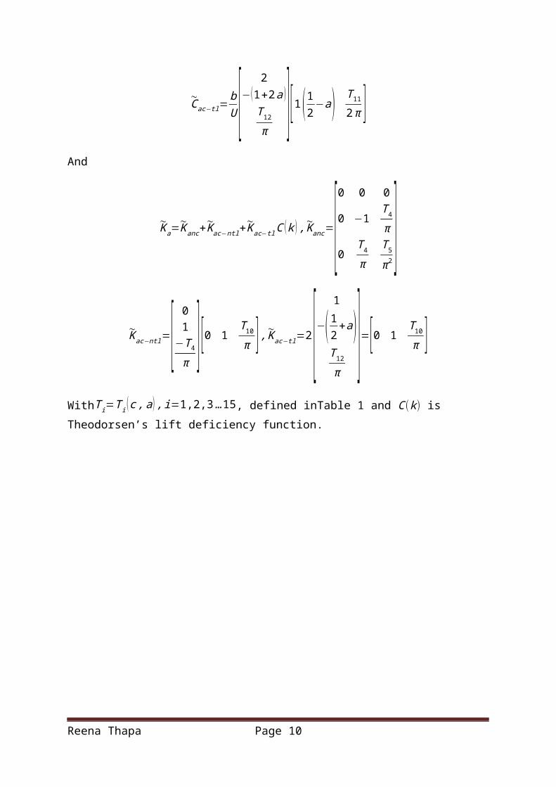
~Cac−tl=bU [ 2
−(1+2 a )T12
π] [1( 1
2−a) T 11
2π ]And
~K a=~K anc+
~K ac−ntl+~K ac−tl C (k ) ,~K anc=[
0 0 0
0 −1T 4
π
0T 4
πT 5
π2]
Reena Thapa Page 7
~Kac−ntl=[ 01
−T 4
π][0 1
T10
π ] ,~K ac−tl=2[1
−( 12+a)T 12
π]=[0 1
T10
π ]
WithT i=T i (c , a ) , i=1,2,3 …15, defined inTable 1 and C (k ) is Theodorsen’s lift deficiency function.
Reena Thapa Page 8
Table 1: Table of Theodorsen’s T-functions,T i , i=1,2,3.3 …,∅ c=cos−1c , c=¿distance of the control surface hinge line from mid-chord in semi-chords,a=¿distance of the elastic axis
from mid-chord in semi-chords.
Also, The equations of motion can also be expressed as:
(M +Sq~M a ) x+(C+Sq~Ca) x+(K+Sq~Ka ) x=− [ LG M G M βG ]T
Where
S=2 π b2 , q=12
ρU2∧x=[ h/b α β ]T
3.Simulation ProcedureStep 1: In order to simulate the governing equations of motion of the two degrees of freedom vibration model, they first were expressed as:
[ h/bα ]=[ 1 xa
xa I a/m b2]−1
+{[LG bM G ]−[kh/m 0
0 k a/mb2][h/bα ]}
This can also be written as:
[ h/bα ]=[ 1 xα
xα rα2 ]
−1
([ LG bM G ]−[ωh 0
2 00 rα
2 ωα 02 ][h /b
α ]) Or as:
[ h/bα ]= 1
ra2−xa
2 [ ra2 −xa
−xa 1 ]−1{[LG b
M G ]−[ωh02 0
0 ra2 ωa 0
2 ][h/bα ]}
≡ 1R−S2 [ R −S
−S 1 ]{[ LG bM G ]−[K 0
0 P] [h/bα ]}
Step 2: Matlab SIMULINK was used to simulate the dynamics of a two-degree of freedom
vibration model with governing equations of motion given by:
[ 1 xα
xα I α /m b2][ h/bα ]+[k h/m 0
0 kα /m b2]+[h /bα ]=[LG b
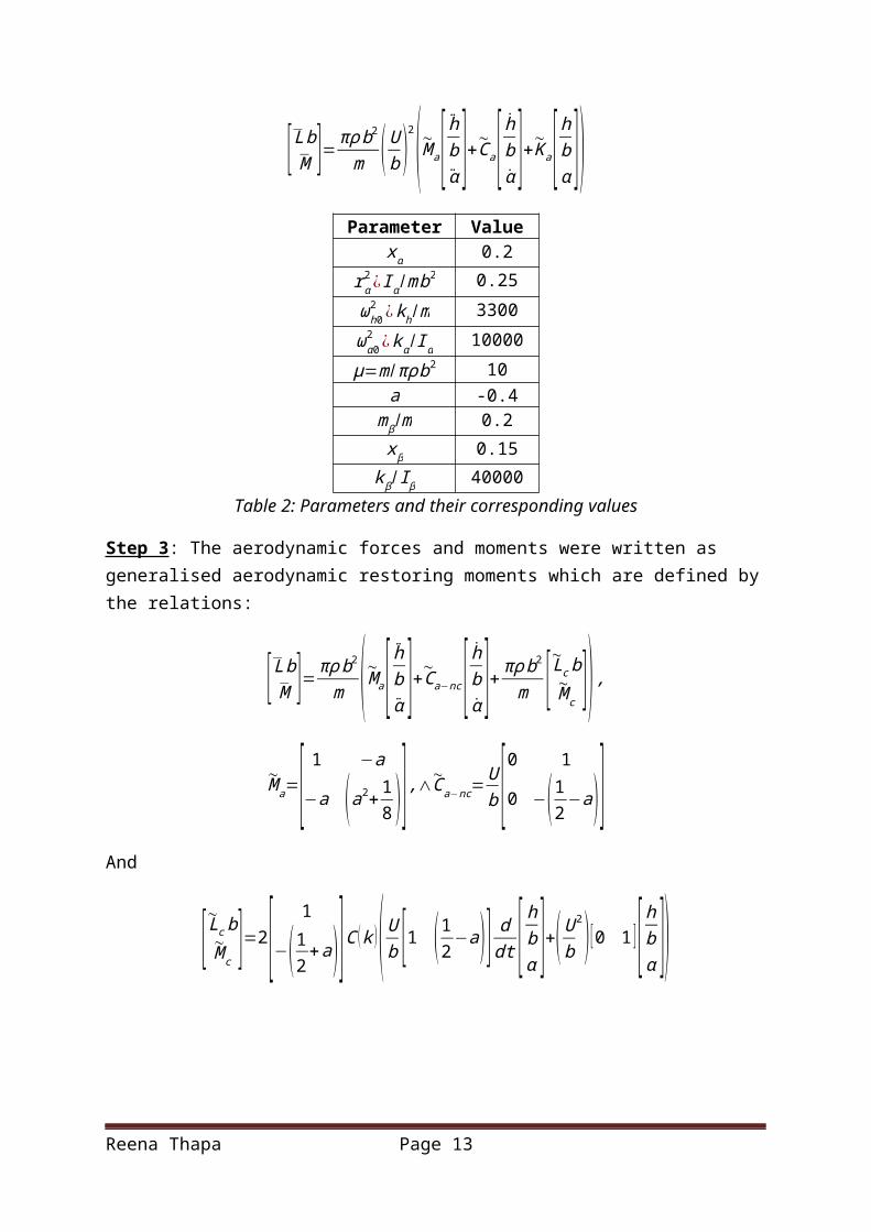
M G ]As listed in Table 2, the parameters with their corresponding values were assumed and any unlisted parameters were appropriately assumed.
Reena Thapa Page 9
[LbM ]= πρb2
m ( Ub )
2(~M a [ hbα ]+~Ca[ h
bα ]+~Ka[ h
bα ])
Parameter Valuexα 0.2
rα2 ¿ Iα /m b2 0.25
ωh02 ¿ kh/m 3300
ωα 02 ¿k α /I α 10000
μ=m /πρ b2 10a -0.4
m β/m 0.2xβ 0.15
k β /I β 40000Table 2: Parameters and their corresponding values
Step 3: The aerodynamic forces and moments were written as generalised aerodynamic restoring moments which are defined by the relations:
[ LbM ]= πρb2
m (~M a [ hbα ]+~Ca−nc[ h
bα ]+ πρ b2
m [~Lc b~M c ]) ,
~M a=[ 1 −a
−a (a2+ 18 )] ,∧~Ca−nc=
Ub [0 1
0 −( 12−a)]
And
[~Lc b~M c ]=2[ 1
−(12+a)]C ( k )(U
b [1 ( 12−a)] d
dt [ hbα ]+(U
b
2
) [ 0 1 ] [ hbα ])
Reena Thapa Page 10
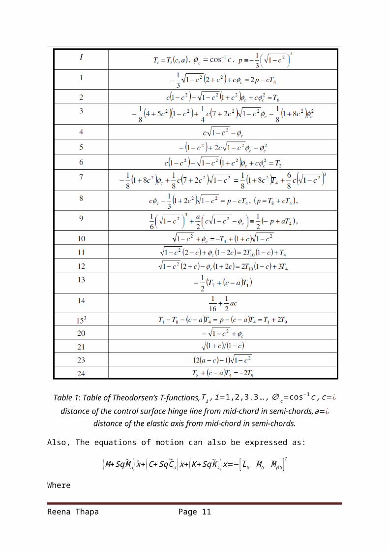
Figure 3.1: The two degree of freedom model without C(k)
Step 4: The Theodoresen function C(k) was assumed as equal to zero and the generalised
aerodynamic restoring moments were included into the SIMULINK model of the governing
dynamics.
C ( k )≈ 1− 0.165 ( ik )ik +0.0455
−0.335 (ik )ik+0.3
The fact that ik is equivalent to bs/U was employed where s is the Laplace transform
variable and using only pure integrators, a SIMULINK model for a system was set up with a
input/output transfer function that is given by:
T ( s )=1− 0.165 s
s+ 0.0455Ub
− 0.335 s
s+ 0.3Ub
Reena Thapa Page 11
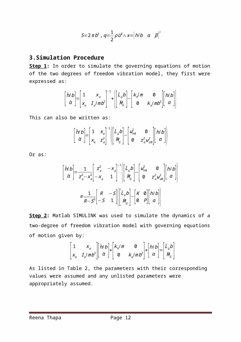
Figure 3.2: The two degree of freedom model with C(k)
1Out1
1s
Integrator1
1s
Integrator
J
Gain3
L
Gain2
0.335
Gain1
0.165
Gain
1In1
Figure 3.3:The block diagram for C(k)
Step 5: A SIMULINK model was developed for four inputs-two output system with inputs
hb
,α , hb∧ α ,and outputs ~Lc b and ~M c.
Step 6 : The sub system developed in Step 4 was employed and the simulation of the two-degrees of freedom flutter model including the generalised aerodynamic restoring moments was carried out.
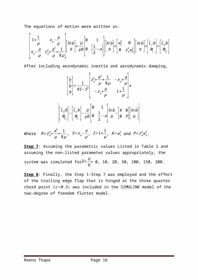
The equations of motion were written as:
Reena Thapa Page 12
[ 1+ 1μ
xα−aμ
xα−aμ
r α2+ a2
μ+ 1
8μ] [h /b
α ]+ Uμb [0 1
0 (12−a) ][ h/b
α ]+[ωh2 0
0 rα2 ωα
2 ] [h /bα ]+[Lc b
M c ]=[LG bM G ]
After including aerodynamic inertia and aerodynamic damping,
[ hbα ]= 1
RI−S2 [rα2 +
a2
μ+
18 μ
−xα+aμ
−xα+aμ
1+ 1μ
] x
{[ LG bM G ]−[ Lc b
M c ]− Uμb [0 1
0 12−a ] h/b
α−[ K 0
0 P] [h/bα ]}
Where R=rα2+ a2
μ+ 1
8 μ, S= xa−
aμ , I=1+ 1
μ , K=ωh2 and P=rα
2 ωα2.
Step 7: Assuming the parametric values Listed in Table 2 and assuming the non-listed
parameter values appropriately, the system was simulated forU =Ub = 0, 10, 20, 50, 100, 150,
200.
Step 8: Finally, the Step 1-Step 7 was employed and the effect of the trailing edge flap that is hinged at the three quarter chord point (c=0.5¿ was included in the SIMULINK model of the two-degree of freedom flutter model.
Figure 3.4: The three degree of freedom model with the trailing edge flap.
Reena Thapa Page 13

4. Results
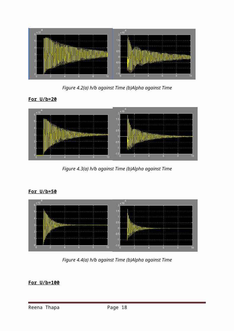
4.1 The Simulation results of two degree of freedom aerofoil model without C(k) For U/b=0
Figure 4.1(a) h/b against Time (b)Alpha against Time
For U/b=10
Figure 4.2(a) h/b against Time (b)Alpha against Time
For U/b=20
Figure 4.3(a) h/b against Time (b)Alpha against Time
For U/b=50
Reena Thapa Page 14
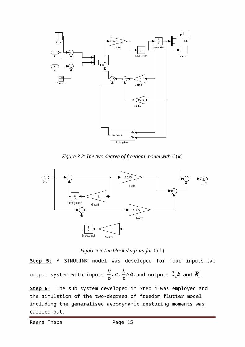
Figure 4.4(a) h/b against Time (b)Alpha against Time
For U/b=100
Figure 4.5(a) h/b against Time (b)Alpha against Time
For U/b=150
Figure 4.6(a) h/b against Time (b)Alpha against Time
Reena Thapa Page 15
For U/b=200
Figure 4.7(a) h/b against Time (b)Alpha against Time
4.2 The Simulation results of two degree aerofoil model with C(k) For U/b=0
Figure 4.8(a) h/b against Time (b)Alpha against Time
For U/b=10
Figure 4.9(a) h/b against Time (b)Alpha against Time
For U/b=50
Reena Thapa Page 16
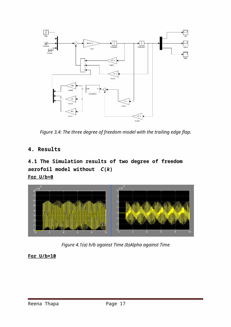
Figure 4.10(a) h/b against Time (b)Alpha against Time
For U/b=100
Figure 4.11(a) h/b against Time (b)Alpha against Time
For U/b=150
Figure 4.12(a) h/b against Time (b)Alpha against Time
Reena Thapa Page 17
For U/b=200
Figure 4.13(a) h/b against Time (b)Alpha against Time
4.3 The Simulation results of three degree of freedom aerofoil with flapFor U/b=0
Figure 4.14: h/b against Time
Figure 4.15:Alpha against Time
Reena Thapa Page 18
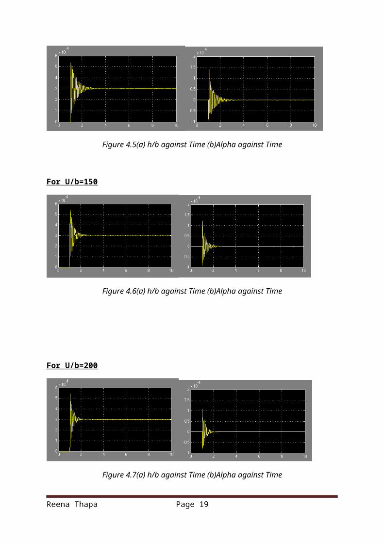
Figure4.16: Beta against Time
For U/b=20
Figure 4.17: h/b against Time
Figure 4.18:Alpha against Time
Reena Thapa Page 19
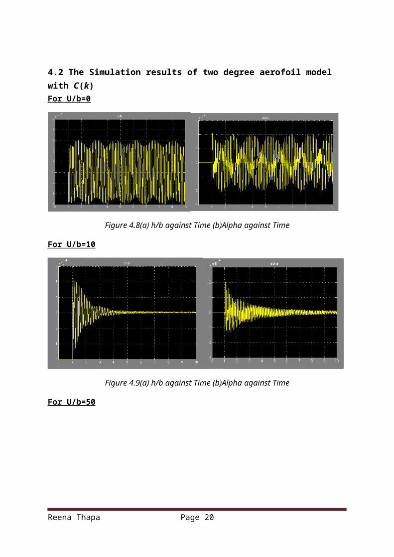
Figure4.19: Beta against Time
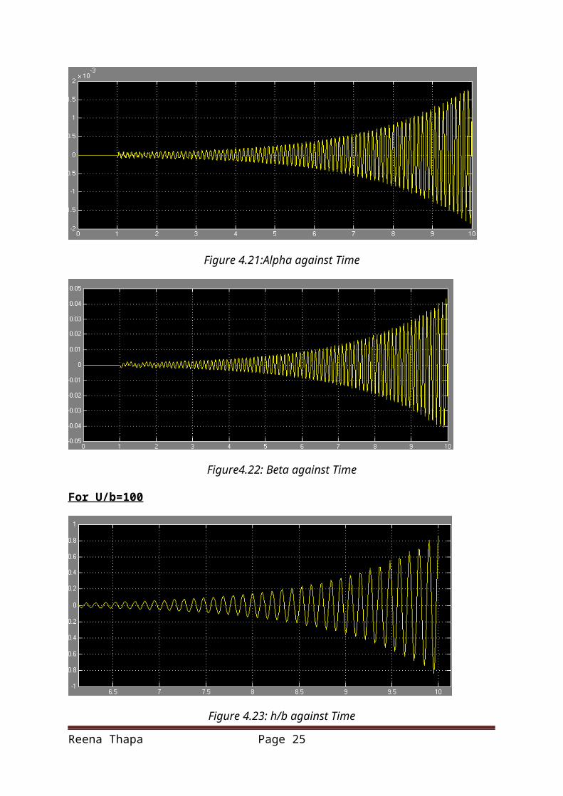
For U/b=50
Figure 4.20: h/b against Time
Figure 4.21:Alpha against Time
Reena Thapa Page 20
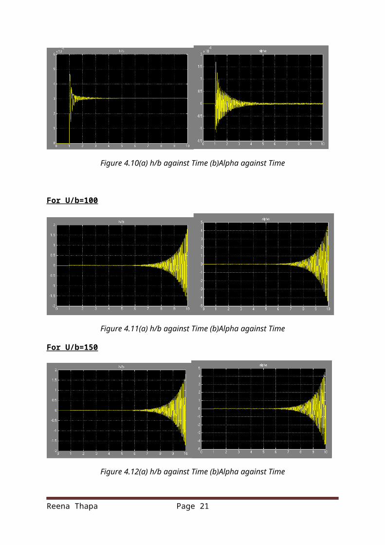
Figure4.22: Beta against Time
For U/b=100
Figure 4.23: h/b against Time
Figure 4.24:Alpha against Time
Reena Thapa Page 21
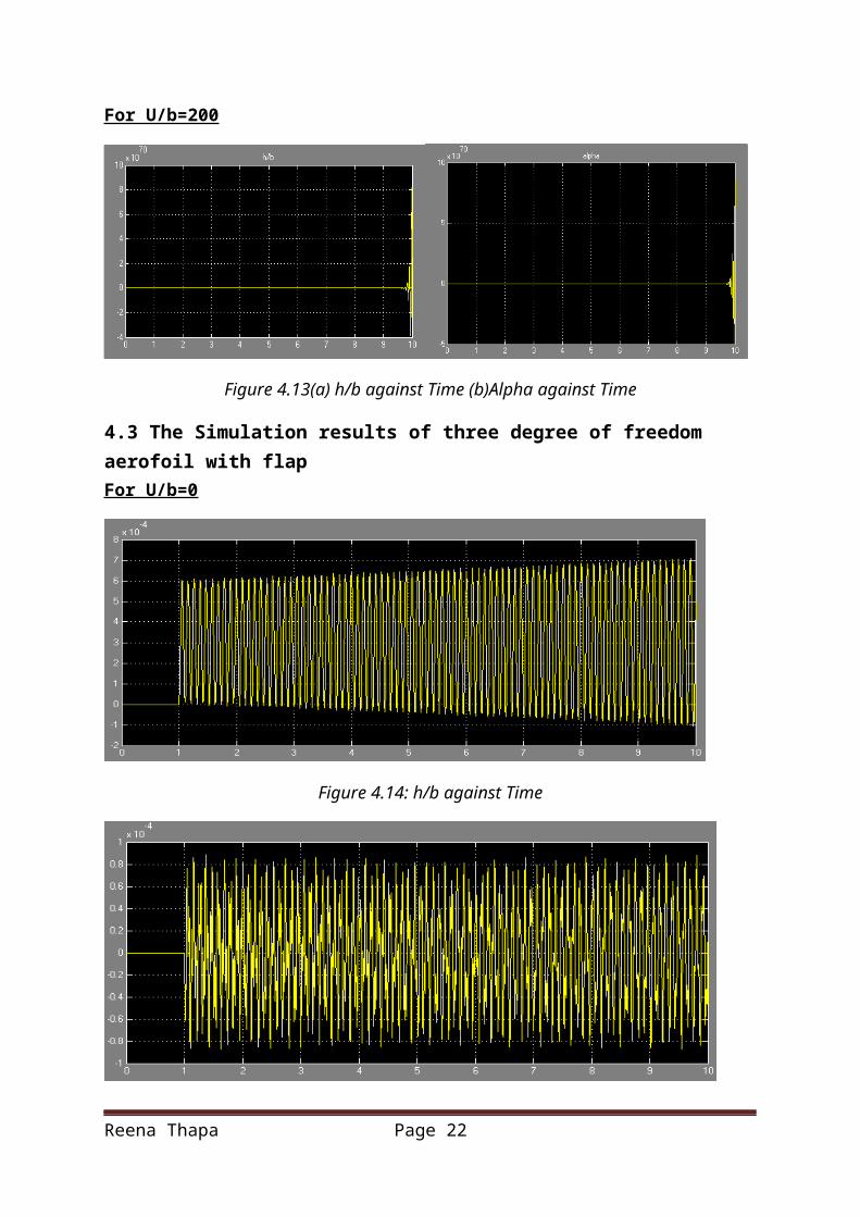
Figure4.25: Beta against Time
For U/b=150
Figure 4.26: h/b against Time
Figure 4.27:Alpha against Time
Reena Thapa Page 22
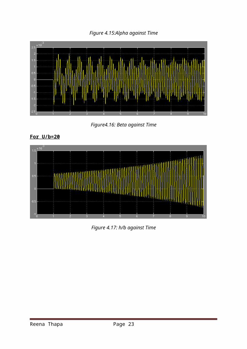
Figure4.28: Beta against Time
5. DiscussionThe graphs from Figure 4.1- Figure 4.28 are the results obtained from the 3 sets of simulations:(1)two degree of freedom aerofoil with C(k) (2)two degree of freedom aerofoil without C(K) and (3) three degree of freedom aerofoil with flap. Each set of results are
obtained for a varying values ofU=Ub = 0, 10, 20, 50, 100, 150, 200. The y-axis consist of
non- dimensional amplitudes caused by translational disturbance, h/b, non-dimensional amplitudes caused by pitch angle disturbance, α and non-dimensional amplitudes caused by the flap angle disturbance, β.
The results in section 4.1 are obtained from first set of simulations when the complex function, C(k) are not considered. Figure 4.1(a) shows the zero amplitudes displacement until 1 s and the amplitude displacement can be observed upto 0.0006 throughout till 10 s when U/b=0. This shows high instability. Figure 4.1(b) shows the amplitude displacement caused by the angle of attack when U/b=0. There is zero displacement until 1 s, after which serious fluctuations in its amplitude displacement can be observed upto a magnitude of 0.0002 throughout till 10 s. In both cases, the instability remains throughout the total time. However, when U/b= 10, the amplitude displacement can be observed up to a 0.00055 at Figure 4.2(a) and upto a 0.0002 at Figure 4.2(b) which dies eventually with time. This is caused by damping and making the system stable eventually with time. As U/b increases, it can be observed that the damping occurs earlier in the system making the system stable.
For the second set of simulations, even though the complex function is considered, the trends of graphs in section 4.2 are similar to that obtained in section 4.1. However the trend changes when U/b=100. The instability begins to occur at 6s which the system fails to dampen. At U/b=200, as seen in Figure 4.13, the instability begins to occur at a much later time i.e. 9.8 s.
Reena Thapa Page 23
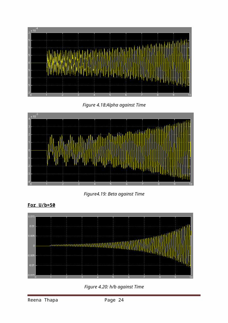
For the third set of simulations, that was run for the three degree of freedom of aerofoil with the trailing edge flap, the instability or flutter can be observed throughout the system as seen from Figure 4.14-4.28. Also the amplitudes are found to be displaced with higher magnitude as U/b increases, indicating the dangerous and unstable vibration regime of the system.
6. ConclusionThe fluttering analysis of the aerofoil was carried out employing three particular cases of simulation for two degrees and three degrees of freedom. In the first set of simulation, Complex function, C(k) was assumed to be zero for the flutter analysis of aerofoil for two degrees of freedom, which appeared to be almost stable. The second set of simulation was carried out which was similar to the first simulation but complex function was considered. As a result, Some instabilities were added to the system due to extra forces and moments. Whereas the set of simulation was operated for the three degree of freedom aerofoil which included the trailing edge flap. This made the system very unstable causing the flutter throughout the system, which can be assumed to be caused by the deflection of the flap by angle β .
7. ReferencesBergami, L.,2008. Aeroservoelastic Stability of a 2D Airfoil Section equipped with a Trailing Edge Flap. Roskilde, Denmark: Technical University of Denmark.
Bisplinghoff, R.L., Carter, A.H. & Halfman, R.L.,1996. Aeroelasticity. Addison-Wesley.
Vepa, R,2014. Computer Aided Simulation Tutorial Exercise. Lab handout. London: Queen Mary University of London.
Reena Thapa Page 24
Reena Thapa Page 25


