EXAMPLE 3 - SCADA Pro · 2018-07-23 · EXAMPLE 3: “Steel Structure” 4 Apart from the RIBBON...

EXAMPLE 3: “Steel Structure”

2

CONTENTS

OVERVIEW ................................................................................................................................................................................ 3

INTRODUCTION ......................................................................................................................................................................... 3

THE NEW INTERFACE ................................................................................................................................................................. 3

1. GENERAL DESCRIPTION .......................................................................................................................................................... 5 1.1 Geometry ...................................................................................................................................................................... 5 1.2 Materials ...................................................................................................................................................................... 5 1.3 Regulations ................................................................................................................................................................... 5 1.4 Sections ........................................................................................................................................................................ 5 1.5 Load – Analysis assumptions ......................................................................................................................................... 6 1.6 Notes ............................................................................................................................................................................ 6

2. DATA INPUT - MODELING ....................................................................................................................................................... 7 2.1 How to start a new project ............................................................................................................................................ 7 2.2 New Project................................................................................................................................................................... 9 2.3 Project Modelling from a 3D dwg file ........................................................................................................................... 10 2.4 Preparing a 3D dwg file ............................................................................................................................................... 11 2.5 Import of the drawing file and sections recognition...................................................................................................... 12 2.6 Footings configuration ................................................................................................................................................ 21

3. LOAD INPUT ........................................................................................................................................................................ 24 3.1 How to insert wind and snow loads automatically in accordance with EC 1: ................................................................. 24

4. ANALYSIS ............................................................................................................................................................................. 32 4.1 How to create an analysis scenario: ............................................................................................................................. 32 4.2 How to run an analysis scenario: ................................................................................................................................. 37 4.3 How to create load combination: ................................................................................................................................. 41

5. POST-PROCESSOR ................................................................................................................................................................ 44 5.1 How to view diagrams and the deformed shapes results: ............................................................................................. 44

6. STEEL MEMBER DESIGN ....................................................................................................................................................... 47 6.1 How to create design scenarios: .................................................................................................................................. 47 6.3 Steel members design:................................................................................................................................................. 53 Merge Elements....................................................................................................................................................................... 53 6.3.1 Cross Section Design: ................................................................................................................................................... 58 6.3.2 Buckling Members Input: ............................................................................................................................................. 60

7. CONNECTIONS ......................................................................................................................................................................... 65 7.1 How to perform steel members’ connection design: ..................................................................................................... 65

8. FOOTING DESIGN................................................................................................................................................................. 68 8.1 How to perform footing design: ................................................................................................................................... 68

9. BILL OF MATERIALS .............................................................................................................................................................. 69 10. DRAWINGS ...................................................................................................................................................................... 70

10.1 How to import the detailing drawings: ......................................................................................................................... 71 11. PRINTING ........................................................................................................................................................................ 73

11.1 How to create the report: ............................................................................................................................................ 73


3

OVERVIEW SCADA Pro new version is a result of more than 40 years of research and development while containing all the innovative capabilities and top-notch tools for the construction business. SCADA Pro utilizes a compact and fully adequate platform for constructing new buildings (analysis and design) or existing ones (check, assessment, and retrofitting). The software employs the Finite Element Method, combining line and plane finite elements in a smooth way. For design purposes, the user is offered all the Eurocodes as well as all the relevant Greek regulations (N.E.A.K, N.K.O.S., E.K.O.S. 2000, E.A.K. 2000, E.A.K. 2003, Old Antiseismic, Method of permissible stresses, KAN.EPE). There are numerous possibilities offered for the modeling of various kind of structures. Structures made of reinforced concrete, steel, timber, masonry, or composite structures are now fully feasible. Several smart operations add on to the practicality and usability of the software. The user can produce the model of a structure no matter how complicated it is, work at ease with the 3D model, process through the steps of analysis and design in a convenient way, up to the conclusion of what initially may seem the most demanding project. SCADA Pro is presented to you as a powerful tool to meet the highest needs of modern civil engineering!

INTRODUCTION The current manual comes as an aid for a new user of SCADA Pro, making the interface of the software as familiar as possible. It consists of several chapters, where one after the other, describes the consecutive steps of a simple example of a loadbearing masonry project. The most useful information is presented, in regards to the best possible understanding of the software commands and logic, as well as the process that has to be followed.

THE NEW INTERFACE The new interface of the SCADA Pro software is based on the RIBBON structure, thus, the several commands and tools are reached neatly. The main idea of the RIBBON structure is the grouping of commands that have small differences and work in the same context, in a prominent position different to each group. This converts the use of a command, from a tedious searching procedure through menus and toolbars, into an easy to remember the chain of two or three clicks of the mouse button.

The user can collect his/her most popular commands

into a new group, for an even faster access. This group remains as it is for future analyses after the program ends. Different commands can be added to it or removed from it, and its placing in the workspace may be altered through the “Customize Quick Access Toolbar” utility.


4

Apart from the RIBBON structure, all the entities that a structure consists of are presented in a tree structure, at the left side of the SCADA Pro main window, either for the whole structure or at each level of the structure. This categorization enhances the use of each entity. When an entity is being chosen by the tree structure, it is highlighted at the graphical interface and the level of the structure that contains this entity is isolated. At the same time, at the right side of the window, the entity’s properties appear. The user can check or modify any of these properties at once. Conversely, the entity can also be chosen at the graphical interface, and automatically it is presented, at the left side in the tree

structure and at the right side with its properties. The right-click mouse button can be very helpful here, since several commands and features, distinct for each entity, can be activated with it.

The “Properties” list that shows up at the right side of the window, not only shows all the properties of the entity shown but can be used for any quick and easy changes, the user wants to make, too.


5

1. GENERAL DESCRIPTION

1.1 Geometry

Current steel structure is a truss created in 3D cad. The upper-structure consists of steel only, while single concrete footings and connecting beams in both directions form the foundation. The final result should look as the following image:

1.2 Materials

For the upper-structure is used steel of quality S275 (Fe430). The modulus of elasticity is Ε=21000kN/cm2 and the Poisson ration is ν=0,30. The specific weight is considered 78,5 kN/m3.

1.3 Regulations

Eurocode 0 (EC0, ENV 1990), for the definition of the load combinations. Eurocode 3 (EC3, ENV 1993), for the design of the steel members. Eurocode 8 (EC8, EN1998), for seismic loads. Ευρωκώδικας 1 (EC1, EN1991), for wind and snow loads. Eurocode 2 (EC2, EN1992), for the footing design.

1.4 Sections

Columns: HEB500 Main Beams: SHS150X8-SHS100X8 Truss Upper: IPE300


6

Truss Lower: IPE300 Truss members: CHS193,7X10 Griders: IPE200 Vetr. Wind bracing: SHS100X5

1.5 Load – Analysis assumptions

Dynamic Spectrum Analisys with pairs of torsional moment of the same direction. The loads in accordance with the method above are: (1) G (dead) (2) Q (live) (3) EX (node loads, seismic forces along ΧΙ axes, derived from dynamic analysis). (4) ΕZ (node loads, seismic forces along ΖΙΙ axes, derived from dynamic analysis). (5) Erx ±(node torsional moments, derived from node seismic forces along ΧΙ axes, offset by the accidental eccentricity ±2eτzi). (6)Erz±(node torsional moments, derived from node seismic forces along ZIΙ ΧΙ axes, offset by the accidental eccentricity ±2eτxi. (7)EY (seismic vertical component –seismic force along y direction- derived from dynamic analysis). For this example we will also include the three following loads: (8) S (snow) (9) W0 (wind along x direction) (10) W90 (wind along z direction) In seismic analysis involved only dead and live loads. Snow and wind loads are considered in separate "simple" static analysis scenario (see Analysis). The values of snow and wind loads in this example will be taken arbitrarily without accurate calculation according to the Eurocode 1, for simplicity. ψ0, ψ1, ψ2 action factors, will be according to EC0.

1.6 Notes

All the commands that will be used in this example (in fact the whole group of the software commands), are analytically described and explained in the User’s Manual of the software.


7

2. DATA INPUT - MODELING

2.1 How to start a new project

SCADA Pro offers several ways to start a new project. Some criteria related to the acceptance of the starting method are: materials, architectural files, floor plan shape, type of elements usage (beam/shell elements) etc.

In this example will be explained in detail the way of using a 3D dwg file for the modeling of a steel structure.

Right after opening the program, the starting dialog form with a group of commands, related to initializing a project, is displayed:

By left clicking on the related icons, one of the following ways, to initialize a project, can be performed:

No matter which way you choose to start a new project, the same form always opens to set the project name and the path of the file, a necessary procedure so that the program commands can work.


8

NOTE: The name of the file can contain up to 8 characters of the Latin alphabet and numbers, without any symbols (/, -, _ ) nor spaces. You can add a description or add some information related to the structure, in the “Info” field.

“new”: It is used when there is no help file in electronic format. The startup is performed in an empty worksheet. The engineer starts with the definition of the

height levels and the sections, and moves on to modeling, using the modeling commands and the snap tools of the program.

“REVIT”: Reading ifc files created by the Autodesk Revit. By using appropriate libraries, SCADA Pro automatically recognizes all the structural elements (columns, beams, slabs, etc.) with their respective properties, generating in this way the ready for the analysis model.

: Reading .xml files Read an .xml file from ARCHLine.XP architectural software.

: Import a cad file and use it as an auxiliary file into the interface or base for

Automatic Level Creation and Automatic Section Identification.

A detailed description of the automatic procedure based on the .acad files is given

in the concrete structure example.


9

“Templates”: SCADA Pro carries a rich library of structure templates for every type of material. The command can be activated either by clicking on one of the startup icons or by accessing the Modeling>Add-ons>Templates. A detailed explanation of this command can be found at the respective chapter of the manual (Chapter 2. Modeling).

concrete shell elements steel

masonry timber connections ( IDEA statiCa)

The most common steel structures

contain continuous frames in one or both directions with duo pitch roof. Stringers, purlins, windbreakers, and front columns may be included. In case of using a template structure, you can perform the entire modeling with one single command! However, in case of more models that are complicated as well, the template command can set the bases to complete the entire modeling faster, just by modifying some of the automatically generated characteristics.

2.2 New Project

Select the related icon and in the dialog window

Set the “Project” name. If you wish, write in the “Info” field, some information related to the project and define the path that your project will be stored to, inside the local disk. Automatically opens the General Parameters window, to set the parameters of the project, such as Material and Regulation, and other general parameters. Set the parameters and press OK.


10

2.3 Project Modelling from a 3D dwg file

This example is intended to educate the user in modeling a steel structure from a 3D dwg file. With the new version of Scada Pro, it is possible to automatically identify the steel sections from a three-dimensional design. More specifically, for the automatic identification of the steel sections, the next steps must be followed:


11

2.4 Preparing a 3D dwg file

For this example, the design steel truss structure of the above image is used. It is a one opening frame structure with six trusses. In the 1st and 5th frame there are vertical wind bracings on both sides, and purlins on the roof.

MAIN DESIGN CONDITIONS:

1. Different layers for each cross section were defined during the design


12

2. Also, at the intersection of the lines, where during the cross-section identification, the model requires the existence of a node, the design was made with segments of lines. More specifically, the figure below shows that at the point where the lower truss element encounters the column, it must be a node, so the line is not continuous but consists of two successive segments.

2.5 Import of the drawing file and sections recognition

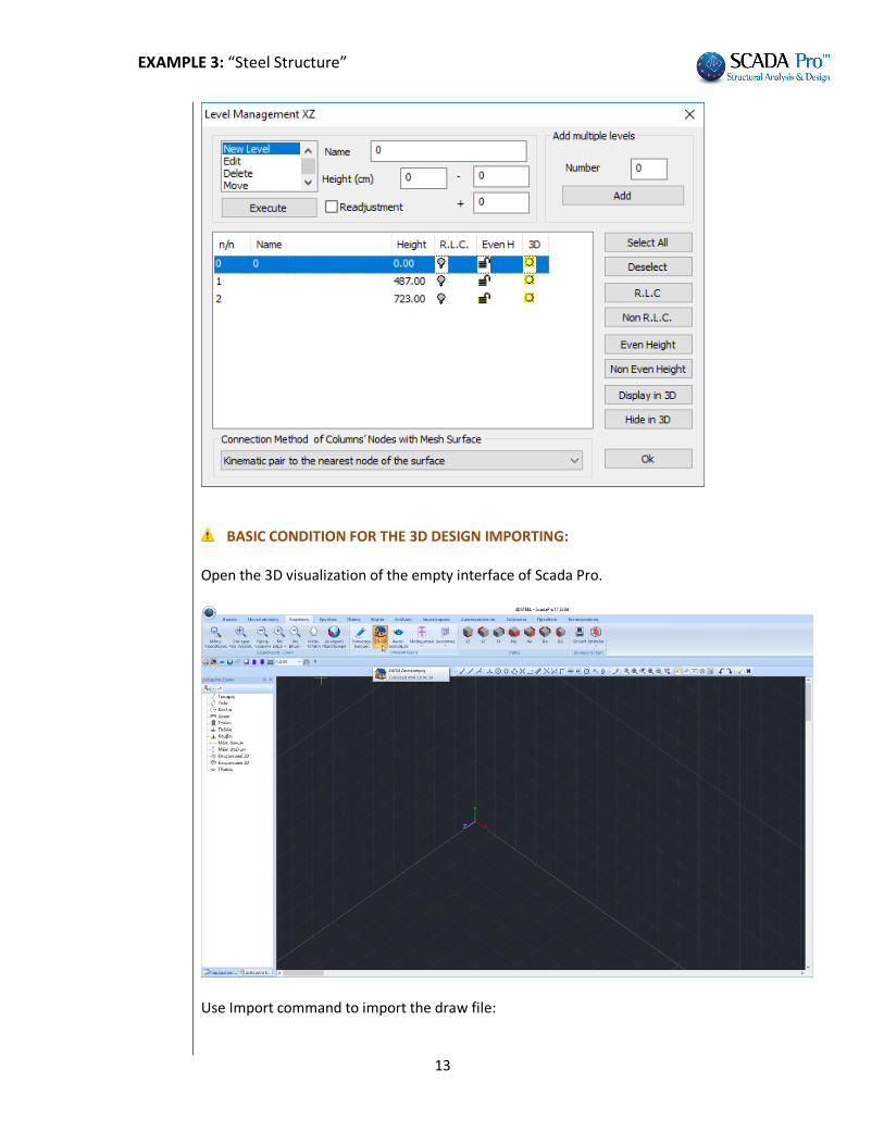
First, give the name of the project, and before the file import, define the levels. In Basic unit, in Layers – Levels

select Level Management XZ and define the levels, deactivating also the Rigid Link Constrain:


13

BASIC CONDITION FOR THE 3D DESIGN IMPORTING: Open the 3D visualization of the empty interface of Scada Pro.

Use Import command to import the draw file:


14

The 3D drawing appears on the 3D interface. From “Basic” and the command group DXF-DWG starts the automatic process of inserting the steel sections: Press Layers to open the Import File Layers including all draw layers and two new commands, Assign Columns Cross-Section and Assign Beam Cross-Section.


15

Select col1 and col2 and press Assign Column Cross-Section

Set the section IPE300, angle 0, quality S275 and layer Steel Columns:


16

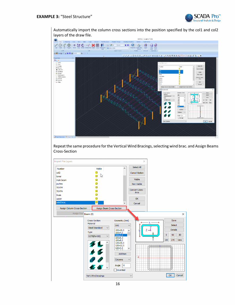
Automatically import the column cross sections into the position specified by the col1 and col2 layers of the draw file.

Repeat the same procedure for the Vertical Wind Bracings, selecting wind brac. and Assign Beams Cross-Section


17

Set SHS100X5 and match the layer Ver. Wind bracings. Ok, and wind bracing cross sections are automatically inserted.

Respectively for the Griders:


18

For the truss elements, set three New Layers in the “Edit Layer” window: -Upper -Lower -Truss To insert all the respective cross sections of the draw layers.

And come to the following model:


19

And activating the virtual view:

ΝΟΤΕ: Truss does not transfer moment, So we have to free the members from the moment.

Using the command “Multiselect Edit” and the Select Group , select Layer “Truss” and Add by Filter and Layer “Lower” and Add by Filter.


20

Ok and right clic to open the Multiselect Edit window. In Element Releases check Mz start and end for all Truss and Lower Layer elements. Apply and Exit to complete.

Left click on a truss element to check that Properties are updated:


21

2.6 Footings configuration

Select Footing in Modeling and define the parameters

Use the 3D visualizzation to insert footings on the bottom of the columns elements.

Correspondingly, for connecting beams, select the cross section and pass them from one node to the other, either in the Mathematical display or Physical. Automatically calculates the beams mathematical model:


22


23

NOTE:

One of the new tools that SCADA Pro offers (after the creation of the mathematical model), is the Footing Predesign:

Which predesigns the footings and may change the dimensions of the footings by the soil interaction stress σ(ΚΝ/m2), the height of the footings Η and the height of the supernatant earth hs.


24

3. LOAD INPUT

3.1 How to insert wind and snow loads automatically by EC 1:

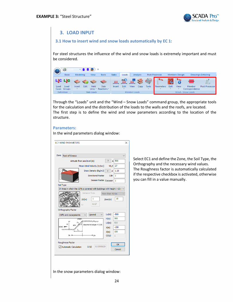
For steel structures the influence of the wind and snow loads is extremely important and must be considered.

Through the “Loads” unit and the “Wind – Snow Loads” command group, the appropriate tools for the calculation and the distribution of the loads to the walls and the roofs, are located. The first step is to define the wind and snow parameters according to the location of the structure.

Parameters: In the wind parameters dialog window:

Select ΕC1 and define the Zone, the Soil Type, the Orthography and the necessary wind values. The Roughness factor is automatically calculated if the respective checkbox is activated, otherwise you can fill in a value manually.

In the snow parameters dialog window:


25

You set the topography which defines the values of the Ce and Ct coefficients, the Zone and the design state.

Edit Walls: Next, through the “Edit” > “Walls”, we define the walls for each direction for the calculation of the Equivalent Wall.

Starting from the wall on the left perpendicular on the wind direction “0”. You define the length (b) and the height (h) for each

wall (Left, Front, Right, Back), by clicking the button and selecting every time with the mouse the two ending points of the wall in the corresponding direction, (model should be viewed in 3D).

Define “h” from the foundation level.

The goal here is to define all the parts of the wall that are perpedincular to the 0 direction of the

wind, with a graphical way, by using the button and pointing to the corners of the wall for the definition of the length (b) and the height (h) of each section, per level.

Next, set the percentage of the openings and click . The program calculates automatically the "Equivalent Wall." Press “OK” command to save the parameters. Repeat for all four directions of the walls.


26

NOTE: The height of the lower wall always defined starting from level 0 even if the steel structure

begins at a higher level. If the front view consists of several walls at one or more levels, press the button "New" and

repeat the above procedure to set the whole face.


27

Edit Roof: Similarly, from “Edit” > “Roof”,

Define the type, the orientation and the dimensions Lo, L1, L2, L3, of the roof by clicking/button and showing with the mouse the four corners of the roof.

View Wind: With the command “View” > “Wind”, you can view for each wind direction the distribution of the wind loads along the height of the structure with the respective Cpe+, Cpe-, Cpi coefficients, for each wall and roof.

View Snow: Similarly, you can use the next command “View” > “Snow”, to view the snow load distribution upon the roof by EC1.

Member Correspondence: to assign the calculated loads to the members, through the influence zones. Select the command and in the dialog box: select a wall, or a roof and define the dimension of the influence zones. In the new version of SCADA Pro, completed and integrated the automatic calculation of influence zones for linear members to make the distribution of wind and snow loads.

Remind that until now the automatic distribution was only for the structures derived from Templates. Now enable this distribution on any surface.

By selecting the command now opens the following dialog box


28

The part on the old definition of the influence zones did not change but added to the right a new part to define the area with three points. The definition always concerns the active area

Better to start either the manual or semi-automatic procedure by pressing the "Members Initialization” button.

Semi-automatic Procedure

Indicate the point graphically with the following particularity: The first two points define the direction by which the automatic calculation of influence

surfaces made for items which are parallel to this direction. Note also that the distribution will be for all linear members belonging to this level and are parallel to the first direction.

After you define the three points, press the "Distribution" button and the program automatically makes the distribution and displays it.

Similarly for the other walls.


29

Concerning the roofs, the definition can be sequentially. First select the roof

, then you must define the individual areas. First define the left slope indicating graphically the 3 points and then the right. The overall result is the following:


30

Finally it is worth noting that if the walls are properly defined there is NO need of more definition. Just select each wall and press «Distribution». The distribution becomes and simultaneously displays on the linear members belonging to this wall.

Same for the flat roofs only.

Post-Processor: This is the last command. On the dialog box, in the “Load attribution” field, there are two units;

-wind loads, four load cases for each direction with a total of 16 load cases -snow loads, three load cases for a typical snowfall, three load cases for an accidental snowfall. The numbers that appear in the fields are the numbers of the load cases.

It is reminded that:

Load Case 1: Dead Load Case 2: Live

And now 16 more cases for wind (from 3 to 18) and 3 for snow (19, 20 and 21). In this example we will not consider the cases of the accidental snowfall.

Select the command to apply the wind and snow loads to the members of the structure, or click

to delete them all. The “Scenarios” field, includes a list with all the possible scenarios of the analysis, which are

automatically created by clicking the button!

Thus SCADA Pro besides of the automatic calculation of the distribution of the wind and snow loads it automatically creates all the analysis scenarios as well.


31

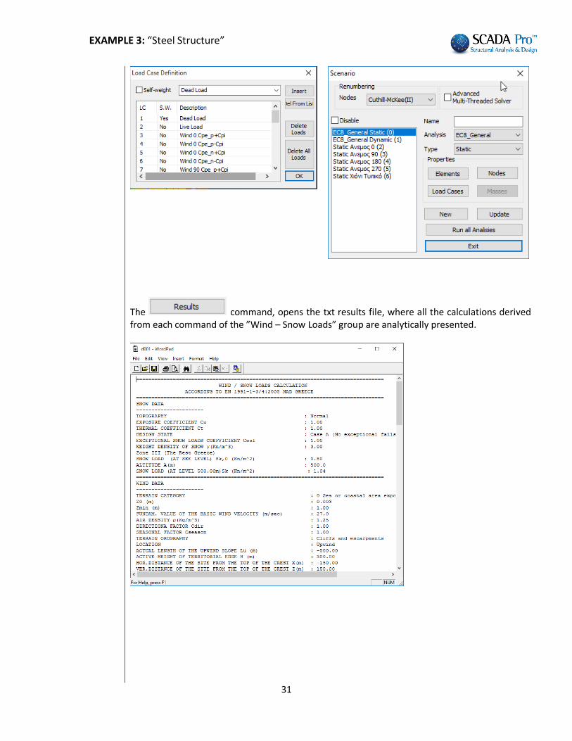
The command, opens the txt results file, where all the calculations derived from each command of the ”Wind – Snow Loads” group are analytically presented.


32

4. ANALYSIS

After the modeling and the distribution of the loads to the members of the structure, the analysis of the structure, by the selected regulation, the creation of the load combination and the results of the checks are next.

4.1 How to create an analysis scenario:

Through the “Analysis” unit, the commands of the “Scenarios” group allow the creation of the analysis scenarios (regulation and analysis type selection) and the execution.

According the selections made in the initial General Parameters window, comes the predefined analysis and members design scenarios.

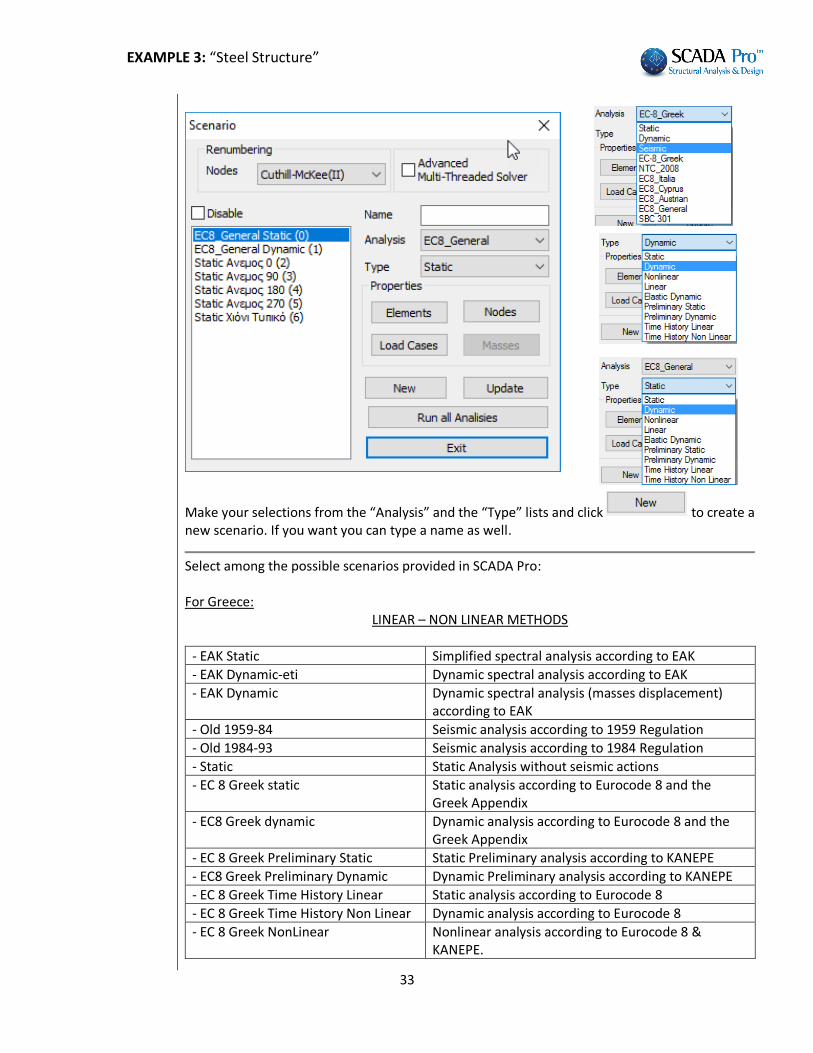
To create more analysis scenarios, select “New”. In the dialog box that opens, besides the predefined ones, you can create as many scenarios as you want.


33

Make your selections from the “Analysis” and the “Type” lists and click to create a new scenario. If you want you can type a name as well.

Select among the possible scenarios provided in SCADA Pro:

For Greece:

LINEAR – NON LINEAR METHODS

- ΕΑΚ Static Simplified spectral analysis according to ΕΑΚ

- ΕΑΚ Dynamic-eti Dynamic spectral analysis according to ΕΑΚ

- ΕΑΚ Dynamic Dynamic spectral analysis (masses displacement) according to ΕΑΚ

- Old 1959-84 Seismic analysis according to 1959 Regulation

- Old 1984-93 Seismic analysis according to 1984 Regulation

- Static Static Analysis without seismic actions

- EC 8 Greek static Static analysis according to Eurocode 8 and the Greek Appendix

- EC8 Greek dynamic Dynamic analysis according to Eurocode 8 and the Greek Appendix

- EC 8 Greek Preliminary Static Static Preliminary analysis according to KANEPE

- EC8 Greek Preliminary Dynamic Dynamic Preliminary analysis according to KANEPE

- EC 8 Greek Time History Linear Static analysis according to Eurocode 8

- EC 8 Greek Time History Non Linear Dynamic analysis according to Eurocode 8

- EC 8 Greek NonLinear Nonlinear analysis according to Eurocode 8 & ΚΑΝΕPΕ.


34

For other countries:

LINEAR – NON LINEAR METHODS

- ΝΤC 2008 Seismic analysis according to the Italian Regulation 2008

- EC8 Italia Seismic analysis according to Eurocode 8 and the Italian Appendix

- EC8 Cyprus Seismic analysis according to Eurocode 8 and the Cyprus Appendix

- EC8 Austrian Seismic analysis according to Eurocode 8 and the Austrian Appendix

- EC8 General Seismic analysis according to Eurocode 8 with no Appendix (enabled typing values and coefficients)

- EC 8 General Non Linear Nonlinear analysis according to Eurocode 8

- SBC 301 Seismic analysis according to Saudi Arabia code (SBC 301)

In this example you’ll only choose the scenarios EC8 dynamic for the earthquake, as well as the scenarios Snow Typical, Wind 0 and Wind 90, which were automatically created as previously explained.

Select the ΕC8 Dynamic. The command Elements, includes the properties modifiers for the beam members.

The program automatically chooses the appropriate inertial modifiers, by the selected regulation while you can modify at any time these modifiers.


35

Select the ΕC8 Dynamic. The command Nodes, opens the following window:

Here you can choose to perform the analysis without considering Rigid Link Constrain at any level even if master nodes exist and consider a fixed base for the whole model even if an elastic foundation is defined. In cases of Dynamic Analysis, if you select “Nodes” and you “open” the springs “Yes”, then you will be able to use the combinations of the dynamic analysis for the design of the footing as well. Select the ΕC8 Dynamic. The command Load Cases, opens the following window:

Where, for each scenario load case (for the current scenario only) on the left column, you match one or more Load Cases (LC) of those that you created.


36

Select the value 1.00 for LC1 (after having selected the category “Dead Loads” – G(1), that are colored blue) and 1.00 for LC2 (after having selected the category “Live Loads” – Q(2), that are colored blue).

The “+” sign next to the load category shows that for the specific category (scenario Load Case) there is a load participation. The maximum “+” signs for each scenario is 4.

Click to update the scenario by the performed modifications. The program fills automatically a unit factor to the corresponding Load Case. Any

modification is acceptable here.

For Static wind and snow scenarios the respective loads participate to the corresponding categories without including the dead and live loads derived from cases LC1 and LC2, since these are already included in the seismic analyzes.


37

When a category is activated the + symbol appears next to it.

NOTE For each scenario, you can activate up to 4 scenario load cases.

4.2 How to run an analysis scenario:

Inside the scenarios list, besides the two predefined scenarios, the scenarios related to wind and snow now exist. Select each scenario and define the corresponding parameters of the selected analysis.

By clicking the “Run” button, depending on the selected scenario, the following dialog box opens: Eurocode scenarios Static scenarios

First of all, select to update the parameters of the current scenario and delete the data of the previously executed analysis.

Then, select to define the parameters of the current scenario.

Depending on the selected scenario, the dialog box differs. In this example having selected the scenario of the Eurocode 8, the dialog box will have the following format:


38

In this dialog box, you enter all the necessary data related to the seismic region, the soil the importance factor, the safety coefficients and the levels of the seismic loads application.

Click the “Seismic Areas” button or type directly the value of coefficient “a”.

Select the importance factor and the coefficient “γι” is automatically filled.

Next define the Spectrum Type and the soil type, so that the horizontal and vertical spectrum coefficients are automatically calculated.

You can modify any of these fields and fill in your very own parameters set.


39

Select the “Spectrum Type” and the “Ductility Class” before you click “Update Spectrum”

Select the “Structural Type” Α) Select the “Structural Type” along X and Z direction to calculate the basic eigenperiod

(in case of structures with a single frame along Χ or/and Ζ direction check the respective checkbox

on the “Bays” group ) Otherwise Β) activate the checkbox to calculate the T1 by the paragraph 4.3.3.2.2. of the EC8 regardless of the structural type

Select the “Structural type” per direction from the list:


40

According to Eurocode the “Behavior Coefficient q” derives from calculations and the “Structural type” must follow specific criteria.

SCADA Pro calculates automatically the q factor and the structural type. The process is explained next:

After having completed all the previously mentioned values, leave the following boxes blank

Choose “Ok” and using the “Automatic procedure” run an initial analysis.

Now, the proposed values for the “Behavior coefficient q” can be found in the “Parameters”

dialog box. The proposed values may be kept or altered (the latter one is an option that could be utilized

from the beginning of the procedure, however, in this occasion the software would not propose any values by EC8).


41

4.3 How to create load combination:

Right after the analysis execution, use the command group “Results”, to create the load combinations (for the EC8 checks and the design) and display the results of the analysis:

The “Combinations” command, opens the “Load Groups Combinations” dialog box where you can create your very own combinations or call the predefined combinations that SCADA Pro has.

After running a scenario analysis, combinations are automatically generated by the program. "Combinations" opens the table with the combinations of the active scenarios. The same results are derived from the "Default Combination" button, which completes the table with the combinations of the active scenario analysis.

The default combinations of the executed analysis, are automatically saved by the program.


42

You can create your combinations without using the "Default", or add more loads of other scenarios and calculate the new combinations either by modifying the defaults, or deleting all "Delete All" and typing other coefficients. The tool “Laod Groups Combinations” works like an Excel file offering possibilities like copy, delete using Ctrl+C, Ctrl+V, Shift and right click. Predefined combinations concerning seismic scenarios. To create combinations of scenarios without seismic loads you can use both automatic and manual mode. The automatic mode requires that the automatic procedure for the calculation and distribution of the loads of wind and snow as well as the automatic creation of the loads and combinations (as in current example) is already done.


43

Concerning the above conditions, it is possible to automatically create wind and snow

combinations by using the command . After running the seismic scenario and all the static scenarios of wind and snow, activate the seismic scenario and choose the command "Combinations". The combinations of the active seismic scenarios are completed automatically. To create automatically the combinations of all

wind and snow loads, press . Automatically the coefficients of all wind and snow scenarios will be filled, offering a complete loads combinations file.

Press to save the file.


44

5. POST-PROCESSOR

5.1 How to view diagrams and the deformed shapes results:

Activate “Post-Processor” to view the deformed shapes of the model for each load case or/and combination scaled accordingly and see the Μ, V, N diagrams for each member as well.

First select “Combinations” and load a combination’s file, depending on the results you want to see. In the dialog box:

Choose a combination from the list that includes the combinations of all the analyses that have been performed, and wait to complete the calculation automatically, or press “Combinations Select”, select the combinations file from the correspondent folder and press "Calculation".

To see the deformed shape of the corresponding eigenvalues, choose a dynamic scenario

.cmb file.

From the list on the right, based on the required results, select: Model or Diagrams Stress-Contours


45

Model + “Deformed”:

Choose from the list the general deformation cause and the next list.

Activate , modify “Magnification” and type in the value of the “Animation Step” to receive a better visualization. On the “Status Bar” check (double click, blue=active, grey=inactive) the type of the visualization of the deformed model.

“Animation” command is a button that activates and deactivates the deformed structure animation, according to the selections made in the “Deformed Model” dialog box.


46

Diagrams – Stress Contours:

In this unit you can see over the members the diagrams of the stress on beam members and the stress/deformation/Reinforcement demand contours, for plate elements. For Linear Members you can see:

tensions , for each , on a , in scale To view to see the six internal forces of a linear member concentrated in one window Select the “2D Member” and left click, for example, on the down right column of the 1st bay.


47

6. STEEL MEMBER DESIGN

After having completed the analysis, checked the results and the deformations the section design follows.

6.1 How to create design scenarios:

Go to “Members Design” section and click “New” to create the scenario by choosing desired regulation.

Type a name, select a type and click New to fill in the Scenarios list.

For this example, a Eurocode scenario was used. Comment: For steel structures the EC3 is applied to every scenario. EC2 regards the analysis method as well as the design method of concrete cross sections. In the field “Design Delete” activate the corresponding checkbox and then press “Apply”, to delete the results of the previous design checks. Repeat using other combinations or parameters or scenarios, etc.


48

6.2 How to define the parameters of the steel members design:

Select from the Scenarios list the scenario that you want to use for the design.

Click “Parameters” to open the following dialog box

Prerequisite for the design is the calculation of the load combinations. The selection of the .cmb file that was stored after the analysis is performed either:

- by selecting from the list which automatically performs the calculation

- or through the command, which is located inside the project folder, you select from the existing ones the desired combination file according to which

the design will be performed and next click the button.


49

In this example, the combination file of the dynamic analysis, including wind and snow will be used.

The Plates, Beams, Columns, Footings, Steel Reinforcement tabs, include the parameters that affect concrete sections. For steel structures, to define the design parameters of the steel sections, select the “Steel” field. The dialog box that opens is divided in two areas: on the left there is a list with all the layers and on the right there is the checks list including all of the respective parameters. First select a layer. Click one from the list, or more using “ctrl”, or all using “Select All”. (By pressing the button “Deselect All” cancel the previous layers’ selection.) Then activate one or more design checks with a tick on the corresponding checkbox and press the corresponding button to specify the parameters. The parameters defined for one layer can be copied to other layers, using the command "Copy". Select a layer define the parameters press “Copy” select another layer press “Paste”.


50

The definition of the design parameters for steel sections is performed per layer. First you select the layer of which the parameters are to be defined, (for example Steel Columns) and for each check category (General, Tension, Shear etc.), you set the respective parameters. As soon as you defined the parameters for one layer, the program gives you the ability to copy these parameters to another layer using the Copy - Paste commands. Suppose you have set all parameters for the layer Steel Columns and you want to pass these parameters to Steel Beams. Activate the check box next to "Default" and automatically all parameters become selected. Then press “Copy”, select layer Steel Beams and press “Paste” (which is now activated). Now all the parameters defined for Steel Columns are defined also for the layer Steel Beams. An alternative method to set the same parameters to all layer including steel sections, is selecting all layer pressing "Select all" button and set once the parameters for each check category. Note that at least one (or more) layer should be selected to set parameters. Next, all the parameters for each category is analytically explained. By clicking the button “GENERAL” the following dialog box opens:

to set the γMi safety factors:

γM0: partial factor for resistance of cross-sections whatever the class is γM1: partial factor for resistance of members to instability assessed by member checks γM2: partial factor for resistance of cross-sections in tension to fracture In the “Limit of Internal” field define an upper limit. Under this value the program will not consider the corresponding stress resultants. These values are recommended by Eurocode.


51

“TENSION”

to define the parameters that correspond to the shear design check as well as the position of the hole check (EC3 §1.8 §3.5):

Specify the spacing of the centers of two consecutive holes, the diameter of the hole and the number of rows of bolt holes. In case of L section specify the parameters on the bottom of the dialog box in the field “Section L”. Here the user defines whether to consider the reduction of the tensile strength of the section due to the bolt holes of the connections or not. The data in the fields of the dialog box are derived from the design checks of the connections. For that reason the verification of the connections must be preceded. The safety factor for all design checks is fixed and equal to one, which means that the program calculates the ratio of the stress resultant versus the resistance. A value of the calculated ratio greater than 1.0 indicates failure.


52

“SHEAR”

Here define if the elements of the selected layer contain stiffeners and what type; web stiffeners or intermediate stiffeners. Also define the spacing between the stiffeners and the type of the connection (rigid or not rigid).

“TORSION”

Here you define whether the structural elements of the selected layer are loaded by a distributed or concentrated torsional moment, or not. If yes you define the load data. You also define the support conditions based on the corresponding figures.


53

For all design checks presented in the figure on the left, define the “Safety Factor” in the dialog box that appears when you click one of the five buttons. The safety factor is the ratio of the resistance value versus the corresponding design value, which is set 1.0 by default.

6.3 Steel members design:

“Steel Design” command group contains commands for the cross-sections design, the buckling resistance and the steel connections design.

Merge Elements

In the new version of the program, added a new command group, which concerns merging of steel (concrete and timber) members for the calculation and buckling and deformation checks display according EC3. IMPORTANT NOTES:

Using this command, is now possible to define correctly, the initial length of the member per

direction to be taken into account in the buckling checks.


54

Until now, this condition was considered defining the length coefficients (see

)

Now, using merging per direction, there is no need for the coefficient process, and merging will be, in most cases, automatically.

Also, note that with the merging process, the buckling length, is calculated correctly, and in the print outs of the results a merged element is printed once with annotation of the individual members that contains.

Basic concepts of buckling along major and minor axies you can find in the User’s Manual Chapter “9. Members Design”

NOTE: Generally, making a rule, we could say that, we consider the merged length Ly in the direction where the local axis y-y is parallel to the supporting elements. While in the other direction, if no supporting elements, Lz is the length of each member. Press Merge Elements command and then Auto:

Merge elements means that, either automatically or manually, the individual parts of a single element, merge in each buckling direction. Meaning that, the buckling length is considered computationally, not the actual length of the element, but the unified from the beginning to the end of the column or beam, respectively. Also, in the presentation of the results, for these merged elements, the worst results display only once and not for each part, as it was so far. Finally, in automatic merging, there is the definition of discontinuity levels, horizontal or vertical, used as merging boundaries of a continuous element. Discontinuity levels are levels that are boundaries of beams and columns, used to break merging in each direction.


55

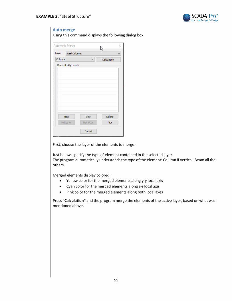
Auto merge Using this command displays the following dialog box

First, choose the layer of the elements to merge. Just below, specify the type of element contained in the selected layer. The program automatically understands the type of the element: Column if vertical, Beam all the others. Merged elements display colored:

Yellow color for the merged elements along y-y local axis

Cyan color for the merged elements along z-z local axis

Pink color for the merged elements along both local axes

Press “Calculation” and the program merge the elements of the active layer, based on what was mentioned above.


56

Discontinuity levels are levels that are boundaries of beams and columns, used to break merging in each direction.

- For the columns, the discontinuity levels are horizontal levels defined by the floor levels. - For the beams, the discontinuity levels are always vertical levels defined by two points.

Predefined limits:

- For the horizontal levels are: the foundation level and the last level. - For the beams are: the vertical limits of the model.

The predefined limits never display in the discontinuity levels list.

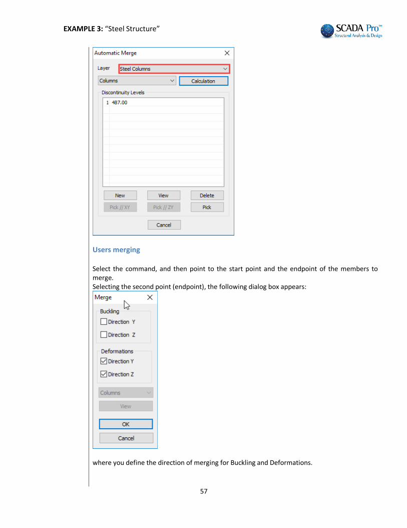
In this example there are three levels 0.00, 487.00 and 725.00 in discontinuity levels list of the columns, only the level 487.00 will be specified by default (that is, only the intermediate level without the limits) considering that, the columns merging will be interrupt at 487.00 cm. The column will merge from 0.00 to 487.00 cm.


57

Users merging Select the command, and then point to the start point and the endpoint of the members to merge. Selecting the second point (endpoint), the following dialog box appears:

where you define the direction of merging for Buckling and Deformations.


58

6.3.1 Cross Section Design:

The command Cross section design is used to check the adequacy of the steel cross-section.

Select this command to open the following dialog box.

The checks are performed for all the elements of the selected layer. The program, for each stress, locates the element with the less favorable value for this stress. The first column contains the layers of the current project and the next columns contain the cross sections of those layers. In this example, the “Steel Columns” layer contains the columns of the structure with the cross section HEB500. Similarly the steel beams belong to the layer “Steel Beams” and the rest of the elements on respective layers. Choose the command “Calculate all” to perform the design checks for each cross section of each layer, for all combinations. Layers with full adequacy of every cross section, will be colored green while the layers that contain at least one cross section with inadequacy will be colored red (which does not mean that all the cross sections of this layer are inadequate necessarily). Select the layer and click “Edit”. On the dialog form you can view in a tabular format the checking results of the cross sections of the selected layer with colored values.


59

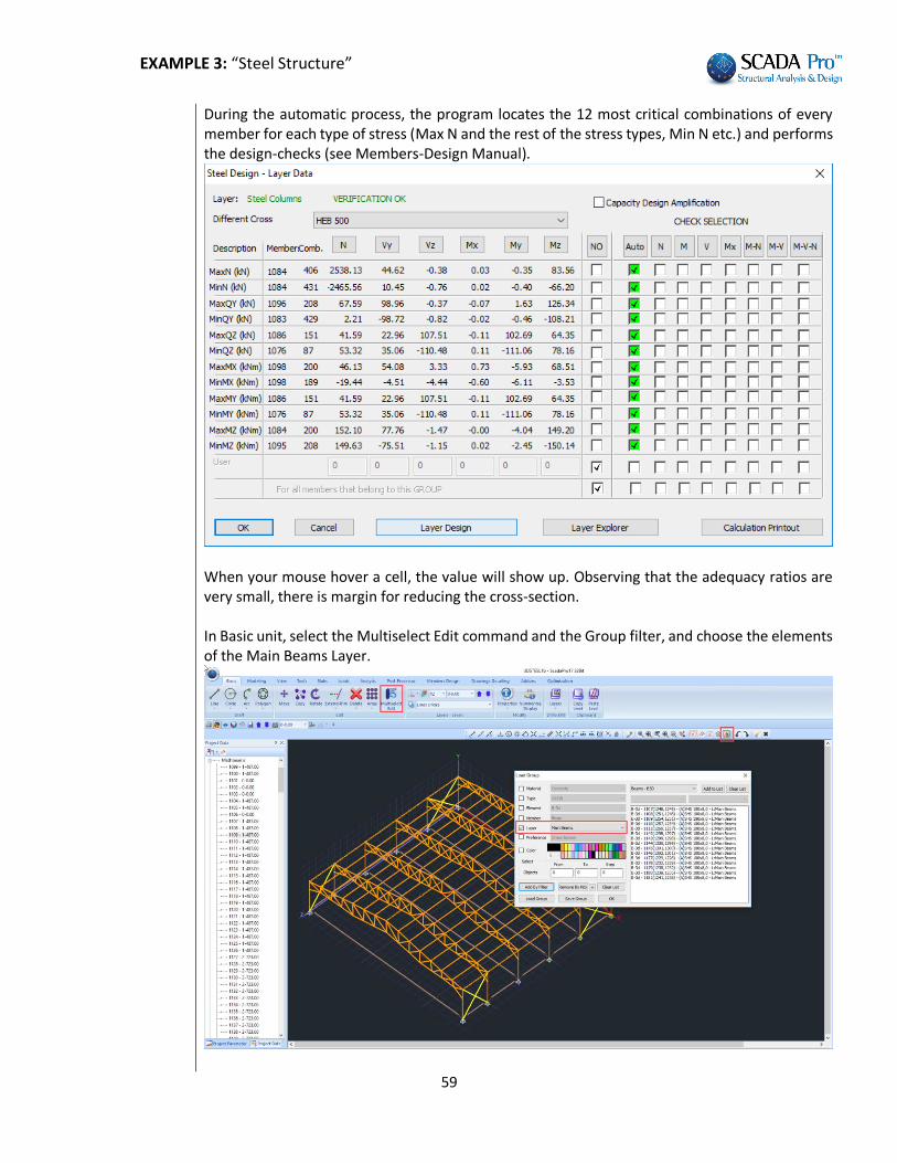
During the automatic process, the program locates the 12 most critical combinations of every member for each type of stress (Max N and the rest of the stress types, Min Ν etc.) and performs the design-checks (see Members-Design Manual).

When your mouse hover a cell, the value will show up. Observing that the adequacy ratios are very small, there is margin for reducing the cross-section. In Basic unit, select the Multiselect Edit command and the Group filter, and choose the elements of the Main Beams Layer.


60

In Cross-Section choose a smaller section, SHS100Χ8.

NOTE: Now you have to run the analyses again to calculate the new intensive forces. Re-run the analyses and reload the combinations in the “Parameters” window, otherwise the section design will be performed by the new cross section but with the previously calculated stresses.

6.3.2 Buckling Members Input:

The buckling resistance check is one of the main design checks for steel structural members. Select the command “Buckling Members Input”, to apply on each member of each layer the following resistance checks:

ULS (Ultimate limit state) SLS (Serviceability limit state)

Flexural Buckling check Member Deflection check

Torsional Flexural Buckling check Node Displacement check

Lateral Buckling check

Lateral Torsional Buckling check

Selecting the command opens the following window:


61

Members Design check is by layer. Select the layer from the drop down list and the "Member" list loads all members of this layer and the cross sections. Define the parameters and If you want to set different parameters to some of them, you can create different “Groups” in the same layer. The program contains two default Groups: "Beams" and "Columns". Select a “Layer” and click on the “Parameters”, and the following dialog box opens:

In the "Group Name" you see the name of the parameter group. If you want to create your group, give a new name and press the button "New Group Creation".


62

In the "Safety Factor" you can set the limit for the program for the design checks: the intensive forces to the respective strength of the member. The default value is 1. The "Limit of internal forces" is the limit that the program uses to take into consideration (or to ignore) the intensive sizes. The rest of the form is divided into four parts, one for each check: For Lateral Buckling check: Because of the “Merging” of the elements, there is no need

anymore to define the Member’s Length. The program will consider the length resulting after merge.

The parameter "Buckling Lengths" depends on the support conditions of the member.

Click on the following button to open the following list and select the appropriate conditions so that the program automatically inserts the corresponding factor.

The icons are divided into two groups: The first group includes icons with a specific factor depending on the member support conditions

Flexural Buckling resistance check:

Activate the checkbox and press The “End Constraints” window, containing the various types of constraints opens. Press one of the first four buttons to automatically calculate the flexural buckling factor:


63

The next parameter refers to the load type of the member at the local axis y, and z respectively. By selecting the corresponding icon, the following options appear: Where you choose the type of Member Loading. For Lateral Torsion Buckling check: activate the checkbox.

NOTE: For the lateral buckling and the lateral torsion buckling resistance check,

the parameters are the same. For Serviceability checks: activate the checkbox “Serviceability Check” and the checkboxes

“Member Deflection Limits” and “Node Displacement Limits”. Then type the corresponding values in each direction, X and Z. For example in the figure on the left, the limits are defined as l/200 and l/150, where l is the member’s length.

Finish the parameters’ input and then press the button "OK" to return to the previous dialog box. To apply the parameters that you set to all members of a layer, select the command "Apply to all members of the Layer".

Activate and click the button "Check in Layer" to check all members of the current layer, with Min and Max of all combinations. The results of the design checks are displayed in the black window that becomes green if it the checks are satisfied of all members of the active layer and red, if not.


64

Activating the option:

, in checks will be taking into account only the maximum and minimum values of the intensive forces resulting from all combinations, excluding the intermediate values so that the process will be completed at noticeably shorter times. Double click ok the colored window, opens the dialog box containing members check summary results:

The first column indicates the number of the member, the second column indicates the cross section and in the next five columns the least favorable ratio of strength and the combination number from which this ratio was resulted is displayed. Greens are the ratios below unity and red the ratios above it. Check all the Layers.


65

7. Connections

7.1 How to perform steel members’ connection design:

The last command of the group command “Steel Members Design” is the “Steel Connections”, used for the steel connections’ design. Select the command and choose one of the following steps: Α) Right click on the screen to open the library that contains all the available steel connections and select the appropriate one. Click on the button “Next Connection Group” to see more connections.

Β) Select with left click the members that you want to connect. Then right click to open a library that contains only the suitable connections for the selected members.


66

Left click to select the column member and then the beam member, and right click to open the library with the four possible types of connection. Select the last one “Beam to Column (Web) Γ” along the main axis. Next set the name of the current connection.

The name must contain only characters from the Latin alphabet and no spaces between the words are allowed.

Then, select the “Member Group Definition (Node)” command and in the dialog box you can add more groups of members with the same connection features (i.e. column – beam) or type your values for the stress resultants Ν, Μ, V for the existing groups. To add groups of members, click into the field “Lower Column” and pick the column 24. Then click into the field “Right Beam” and pick the beam 153 (or just enter the numbers in the corresponding fields) and then click the button “Add”.


67

Use this dialog box for the design of steel connections with the same type and the same cross-sections in total.

The program calculates automatically the forces and proceeds with connection’s design, based on the less favorable load combination. So you don’t have to guess the point of your structure, where the less favorable beam - column connection in the minor axis will be developed. Furthermore, if this connection is satisfied, then all the other connections with the same type will be automatically satisfied, too.

At the end, click “Exit” and select the command “Edit Connections (Geometry/Checks)”. In the new dialog box you can define the type and the geometry of the specific connection. Select the type and enter the geometrical parameters of the cross-section or create your connection. First the program performs the geometrical checks of the connection (e.g. if the bolts are located too close to the edge of the plate). If there is a problem, the corresponding error message appears in the field on the right. In the specific connection, change the distance e1 from 10 to 15 cm and then click again the button "Calculation (Combinations)".

Click the button “3D” to see a three-dimensional representation of the connection that is updated as you change the parameters. The buttons “1”, “2”, “3” are used for the display of the two side views (1 & 2) and the plan view (3). The button “Σ/Κ” is used for the display of the three-dimensional representation of the welds and bolts.


68

If the geometrical checks are satisfied, the program calculates and displays all Eurocode 3 design checks for the connection. Click “Simplified” to see the results. Green fonts means adequacy and red failure. If all checks are satisfied the program will be able to save the connection and generate the drawings automatically. Otherwise the procedure will stop and you need to change some values of the connection to continue. To read the main results click the button “Results” and for all the results, click the button “Exploration”. The displayed *txt files are those generated by the program for the printout. Click “Save” and then “Exit” to return to the connections’ window.

8. FOOTING DESIGN

8.1 How to perform footing design:

As soon as you complete the connection design, you can move on to the footing design. The “Footing” command group contains commands for footing design check, design calculation, editing and the respective results.

Select the command “Check Reinforcement>Overall“ to perform the design checks for all the footings on the current level. The color of the node indicates that the design checks of the footing:

were satisfied or failed. Necessary precondition for the footing designing, is the columns designing in level 1.


69

9. BILL OF MATERIALS

The “Bill of Materials” command group contains the commands related to the estimation of the materials’ quantities and the corresponding cost.

Steel Cross Sections: It calculates the quantity of the structural steel. “Analytical”: per element and cross section concerning the length (m), weight in Kg (per m or in total); “Summary”.

SCADA Pro gives you the ability to have analytic bills of materials for each steel cross section per member or aggregated bills per section category.


70

Press “Results File (Bill of Materials)” to attach the Calculation Printout.

10. DRAWINGS

Since the design and reinforcement of the structural elements of the concrete structures or the design of steel connections of the steel structures have been completed, you can open, modify and finally produce all the drawings in the "Drawing-Detailings” Ribbon. The “Drawing-Detailings” Ribbon incorporates a drawing application in the interface.


71

10.1 How to import the detailing drawings:

The automatically created drawings of the created connections are located inside the folder of the project: C:\scadapro\ “project1” \scades_Synd\sxedia

Use the command to open these drawings inside the SCADA Pro environment: Selecting “Import” command opens the following dialog box for choosing the project’s folder. Then select:

In List files of Type: select “Scada connection *.con”

(In Directories: find the pathC:\scadapro\“STEEL” \scades_Synd\sxedia)


72

Next choose the considered name of the connection (so that it turns blue), click “ok” and finally click inside the desktop at the desired insertion point. In this way three views of the selected connection are created.


73

Follow the previously described procedure to create and import over 120 different type of connections that the program covers. To create the respective views of the model in total you must follow a different procedure.

Click the “Export” command of the main menu to export your drawing in a *.dwg format. In the “Save As” field select the folder of your project and give a name to the exported file and in the “save as type” field select the 3D_dwg Files (*.DWG) format.

Next, if you open the exported *.dwg file using the autocad you’ll notice that the whole structure is exported as a 3D model including the name of each cross-section. Since now you are working in AutoCAD environment you can create any view of your model that you want and even apply photοrealism commands.

11.PRINTING

11.1 How to create the report:

To create the report, open the unit “ADDONS” and select the command “Print”. In the “Calculation’s Printout” dialog form, on the left there are the available for printing units. To add a unit to the printing list (located on the right) double click on it. For this example, select the units that you wish to print and click the “Project Report” button. The preview printing file is automatically opened.


74

Through this environment, you can save your report under .pdf, or .doc, .excel, or .xml format and modify further the exported result if you wish.

Through this simple example you got familiar with some of the most important commands of SCADA Pro. Working with the program you will discover that it has unlimited modeling and design potentials to perform even the most complicated analysis.


75

Date post:	23-Mar-2020
Category:	Documents
Upload:	others
View:	2 times
Download:	0 times

EXAMPLE 3 - SCADA Pro · 2018-07-23 · EXAMPLE 3: “Steel Structure” 4 Apart from the RIBBON...

Documents