(C.Bina, 9/2011) From thermodynamics to geodynamics: An overview of the geophysical thermodynamics of phase relations Craig R. Bina Dept. of Earth and Planetary Sciences Northwestern University Evanston, Illinois, U.S.A. Katedra geofyziky Matematicko-fyzikální fakulta Univerzita Karlova v Praze přednášky na podzim 2011 1. lekce 12.10.
Transcript
(C.Bina, 9/2011)
From thermodynamics to geodynamics:An overview of the geophysical thermodynamics
of phase relations
Craig R. Bina
Dept. of Earth and Planetary SciencesNorthwestern UniversityEvanston, Illinois, U.S.A.
Katedra geofyzikyMatematicko-fyzikální fakultaUniverzita Karlova v Praze
přednášky na podzim 20111. lekce 12.10.
(C.Bina, 9/2011)
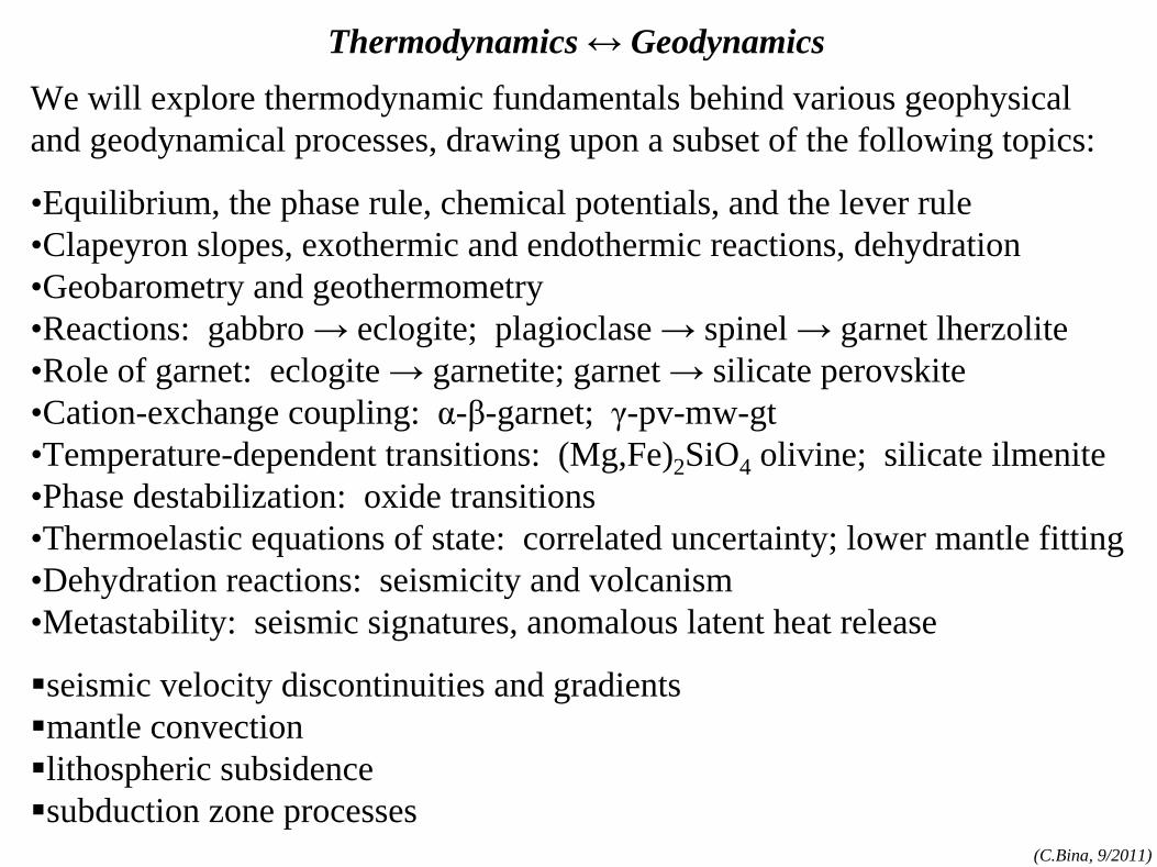
Thermodynamics ↔ GeodynamicsWe will explore thermodynamic fundamentals behind various geophysical and geodynamical processes, drawing upon a subset of the following topics:
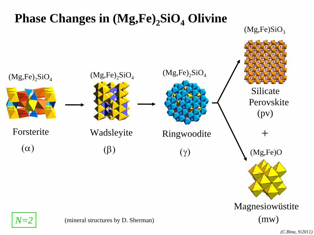
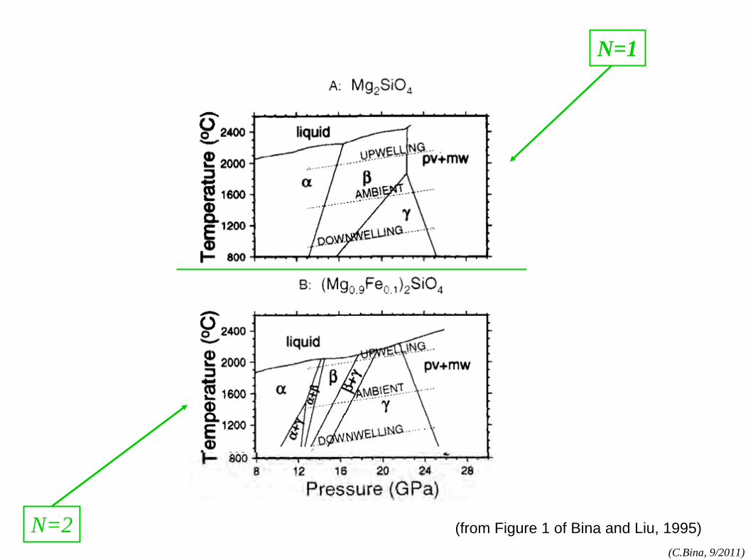
•Equilibrium, the phase rule, chemical potentials, and the lever rule•Clapeyron slopes, exothermic and endothermic reactions, dehydration•Geobarometry and geothermometry•Reactions: gabbro → eclogite; plagioclase → spinel → garnet lherzolite•Role of garnet: eclogite → garnetite; garnet → silicate perovskite•Cation-exchange coupling: α-β-garnet; γ-pv-mw-gt•Temperature-dependent transitions: (Mg,Fe)2
seismic velocity discontinuities and gradientsmantle convectionlithospheric subsidencesubduction zone processes
(C.Bina, 9/2011)
You are welcome to interrupt and ask questions!Some discussion will make these lectures more interesting.
Unfortunately, I do not know everyone’s background in thermodynamics.So, I will spend the first lecture reviewing some of the fundamentals.This part will be rather mathematical (primarily following the approach of Callen [1960, 1985]), and probably we will not begin to discuss interesting geological and geophysical examples until the next lectures.
After each lecture, I will post some notes (PDF) at: http://ajisai.earth.northwestern.edu/private/karel2011/
Welcome
(C.Bina, 9/2011)
An Apology
Many of the figures I have used to illustrate these various ideas are drawn from my own work or from that of my colleagues. This is simply because I have convenient access to these particular figures. Many other scientists have contributed far more to the study of most of these topics. I offer my apologies for not having used more of their figures instead.
(C.Bina, 9/2011)
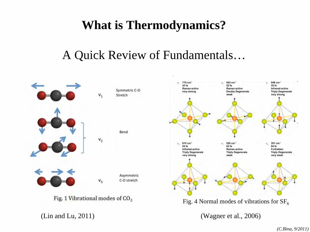
What is Thermodynamics?
A Quick Review of Fundamentals…
(Lin and Lu, 2011) (Wagner et al., 2006)
Fig. 4 Normal modes of vibrations for SF6
(C.Bina, 9/2011)
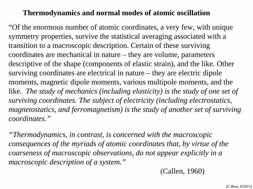
Thermodynamics and normal modes of atomic oscillation
“Of the enormous number of atomic coordinates, a very few, with unique symmetry properties, survive the statistical averaging associated with a transition to a macroscopic description. Certain of these surviving coordinates are mechanical in nature – they are volume, parameters descriptive of the shape (components of elastic strain), and the like. Other surviving coordinates are electrical in nature – they are electric dipole moments, magnetic dipole moments, various multipole moments, and the like. The study of mechanics (including elasticity) is the study of one set of surviving coordinates. The subject of electricity (including electrostatics, magnetostatics, and ferromagnetism) is the study of another set of surviving coordinates.”
“Thermodynamics, in contrast, is concerned with the macroscopic consequences of the myriads of atomic coordinates that, by virtue of the coarseness of macroscopic observations, do not appear explicitly in a macroscopic description of a system.”
(Callen, 1960)
(C.Bina, 9/2011)
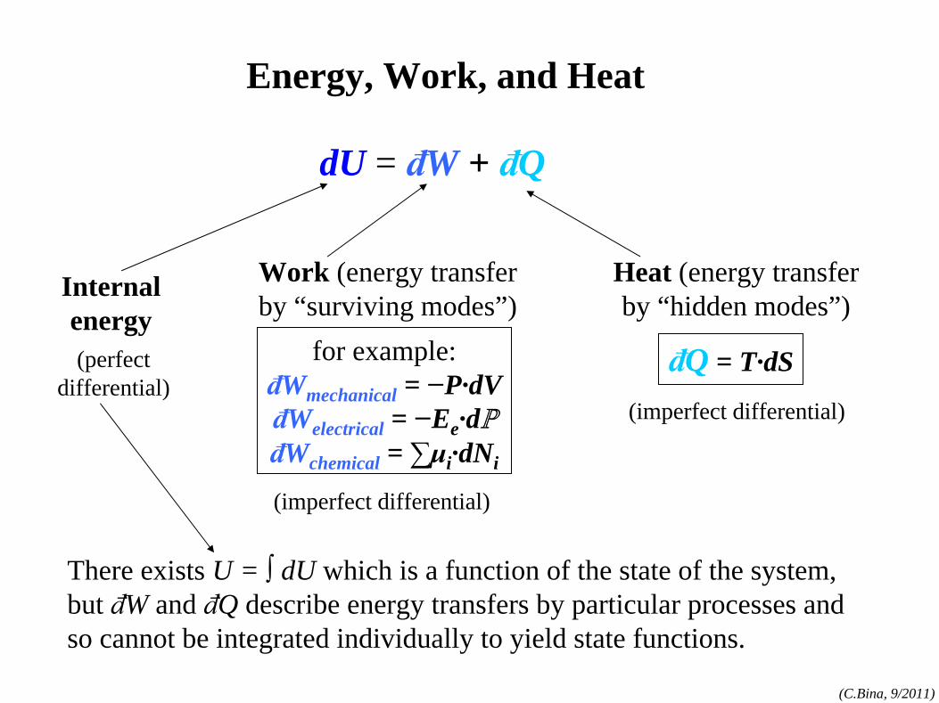
dU = đW + đQ
for example:đWmechanical
= −P·dVđWelectrical
= −Ee ·dℙ
đWchemical = ∑μi
·dNi
Work (energy transfer by “surviving modes”)
Heat (energy transfer by “hidden modes”)
đQ = T·dS
Internal energy
(imperfect differential)
(imperfect differential)
(perfect differential)
There exists U = ∫ dU which is a function of the state of the system, but đW and đQ describe energy transfers by particular processes and so cannot be integrated individually to yield state functions.
Energy, Work, and Heat
(C.Bina, 9/2011)
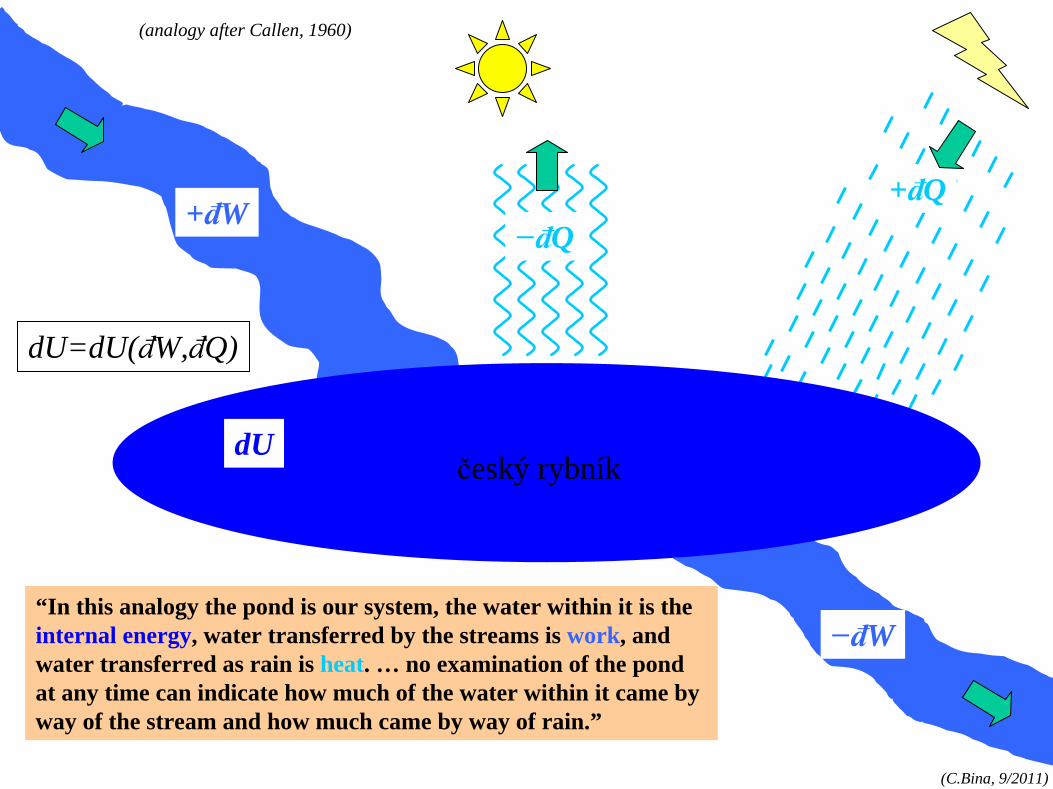
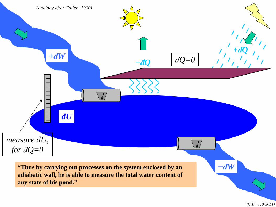
“In this analogy the pond is our system, the water within it is the internal energy, water transferred by the streams is work, and water transferred as rain is heat. … no examination of the pond at any time can indicate how much of the water within it came by way of the stream and how much came by way of rain.”
+đW+đQ
dU
−đW
−đQ
(analogy after Callen, 1960)
dU=dU(đW,đQ)
český rybník
(C.Bina, 9/2011)
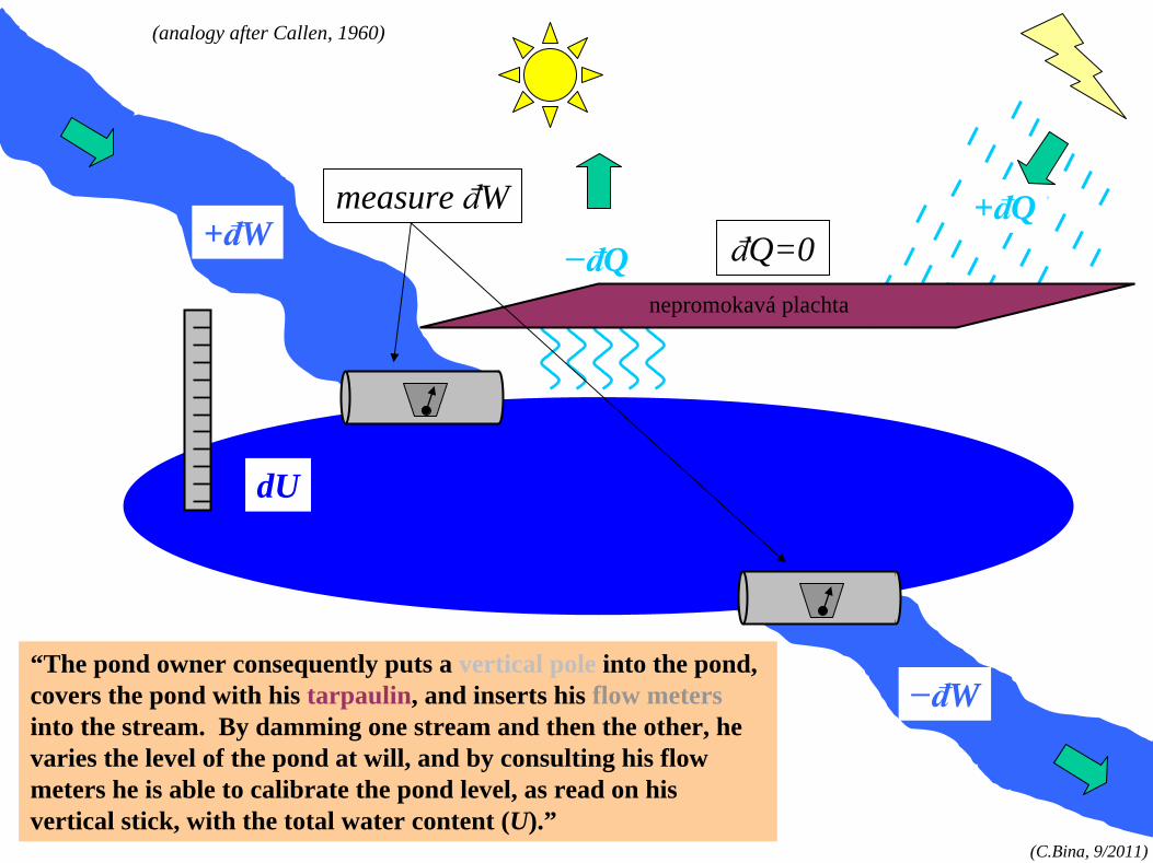
“The pond owner consequently puts a vertical pole into the pond, covers the pond with his tarpaulin, and inserts his flow meters into the stream. By damming one stream and then the other, he varies the level of the pond at will, and by consulting his flow meters he is able to calibrate the pond level, as read on his vertical stick, with the total water content (U).”
+đW+đQ
dU
−đW
−đQ
(analogy after Callen, 1960)
measure đWđQ=0
nepromokavá plachta
(C.Bina, 9/2011)
“Thus by carrying out processes on the system enclosed by an adiabatic wall, he is able to measure the total water content of any state of his pond.”
+đW+đQ
dU
−đW
−đQ
(analogy after Callen, 1960)
đQ=0
measure dU, for đQ=0
(C.Bina, 9/2011)
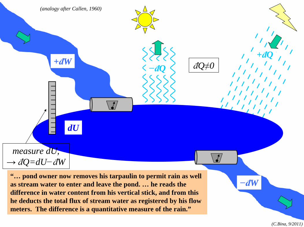
“… pond owner now removes his tarpaulin to permit rain as well as stream water to enter and leave the pond. … he reads the difference in water content from his vertical stick, and from this he deducts the total flux of stream water as registered by his flow meters. The difference is a quantitative measure of the rain.”
(analogy after Callen, 1960)
+đW+đQ
dU
−đW
−đQ
measure dU,→ đQ=dU−đW
đQ≠0
(C.Bina, 9/2011)
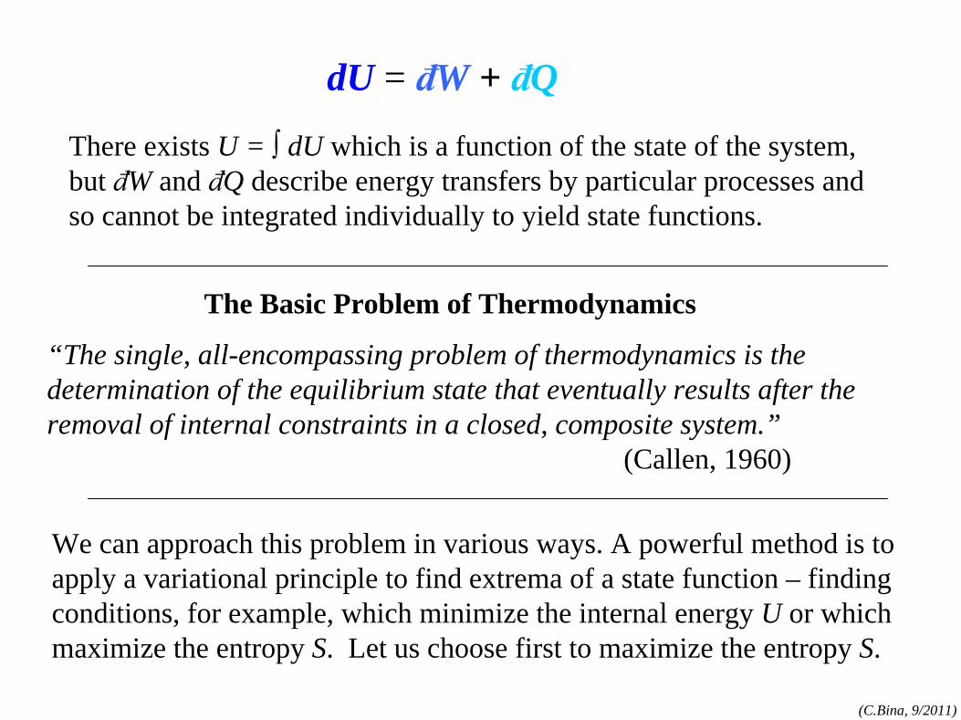
dU = đW + đQ
There exists U = ∫ dU which is a function of the state of the system, but đW and đQ describe energy transfers by particular processes and so cannot be integrated individually to yield state functions.
The Basic Problem of Thermodynamics
“The single, all-encompassing problem of thermodynamics is the determination of the equilibrium state that eventually results after the removal of internal constraints in a closed, composite system.”
(Callen, 1960)
We can approach this problem in various ways. A powerful method is to apply a variational principle to find extrema of a state function – finding conditions, for example, which minimize the internal energy U or which maximize the entropy S. Let us choose first to maximize the entropy S.
(C.Bina, 9/2011)
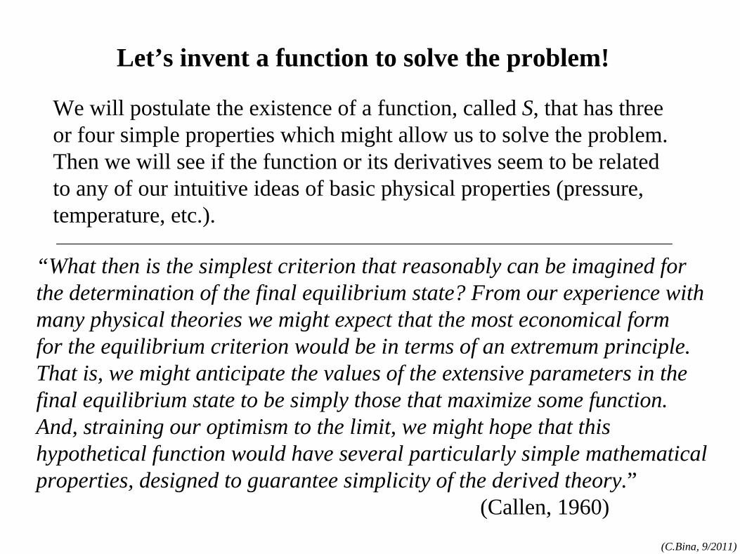
We will postulate the existence of a function, called S, that has three or four simple properties which might allow us to solve the problem. Then we will see if the function or its derivatives seem to be related to any of our intuitive ideas of basic physical properties (pressure, temperature, etc.).
“What then is the simplest criterion that reasonably can be imagined forthe determination of the final equilibrium state? From our experience withmany physical theories we might expect that the most economical formfor the equilibrium criterion would be in terms of an extremum principle.That is, we might anticipate the values of the extensive parameters in thefinal equilibrium state to be simply those that maximize some function.And, straining our optimism to the limit, we might hope that thishypothetical function would have several particularly simple mathematicalproperties, designed to guarantee simplicity of the derived theory.”
(Callen, 1960)
Let’s invent a function to solve the problem!
(C.Bina, 9/2011)
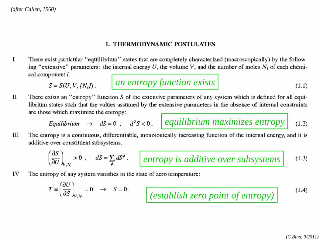
an entropy function exists
equilibrium maximizes entropy
entropy is additive over subsystems
(establish zero point of entropy)
(after Callen, 1960)
(C.Bina, 9/2011)
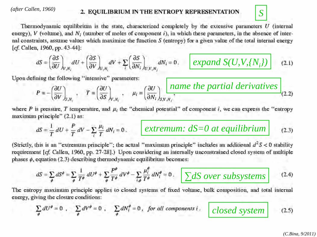
expand S(U,V,{Ni })
extremum: dS=0 at equilibrium
∑dS over subsystems
closed system
S
name the partial derivatives
(after Callen, 1960)
(C.Bina, 9/2011)
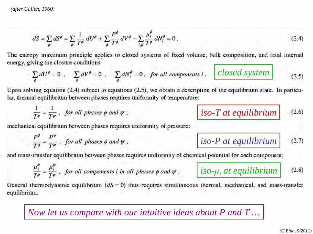
closed system
iso-T at equilibrium
iso-P at equilibrium
iso-μi at equilibrium
Now let us compare with our intuitive ideas about P and T …
(after Callen, 1960)
(C.Bina, 9/2011)
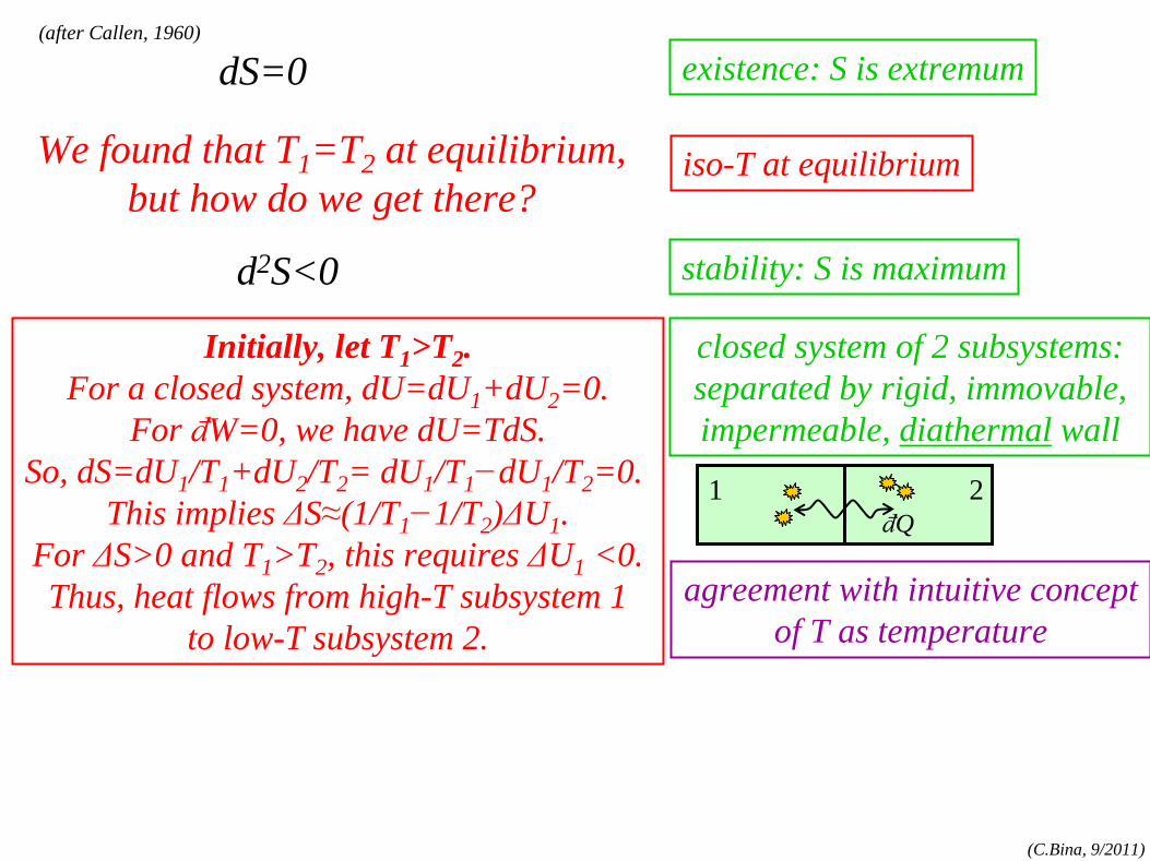
stability: S is maximum
iso-T at equilibrium
d2S<0
We found that T1 =T2
at equilibrium,but how do we get there?
existence: S is extremumdS=0
Initially, let T1 >T2
.For a closed system, dU=dU1
+dU2 =0.
For đW=0, we have dU=TdS.So, dS=dU1
/T1 +dU2
/T2 = dU1
/T1 −dU1
/T2 =0.
This implies ΔS≈(1/T1 −1/T2
)ΔU1 .
For ΔS>0 and T1 >T2
, this requires ΔU1 <0.
Thus, heat flows from high-T subsystem 1to low-T subsystem 2.
closed system of 2 subsystems: separated by rigid, immovable, impermeable, diathermal wall
agreement with intuitive concept of T as temperature
1 2đQ
(after Callen, 1960)
(C.Bina, 9/2011)
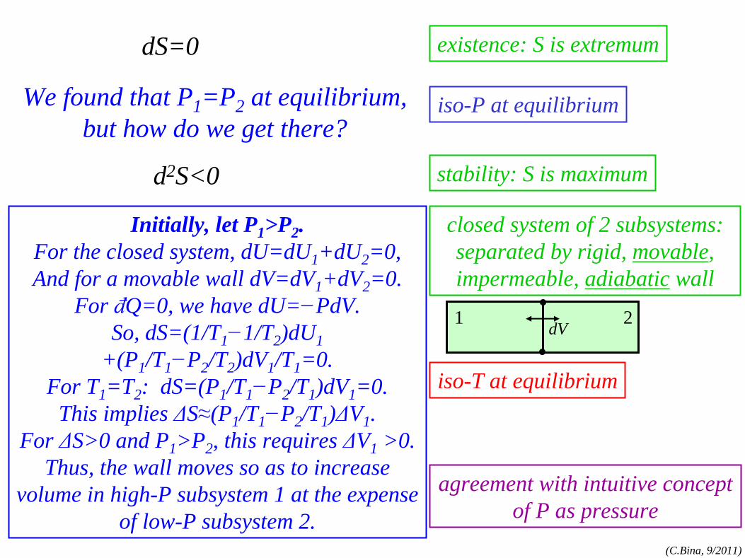
stability: S is maximum
iso-P at equilibrium
d2S<0
We found that P1 =P2
at equilibrium,but how do we get there?
existence: S is extremumdS=0
Initially, let P1 >P2
.For the closed system, dU=dU1
+dU2 =0,
And for a movable wall dV=dV1 +dV2
=0.For đQ=0, we have dU=−PdV.
So, dS=(1/T1 −1/T2
)dU1+(P1
/T1 −P2
/T2 )dV1
/T1 =0.
For T1 =T2
: dS=(P1 /T1 −P2
/T1 )dV1
=0.This implies ΔS≈(P1
/T1 −P2
/T1 )ΔV1
.For ΔS>0 and P1
>P2 , this requires ΔV1
>0.Thus, the wall moves so as to increase
volume in high-P subsystem 1 at the expenseof low-P subsystem 2.
closed system of 2 subsystems: separated by rigid, movable, impermeable, adiabatic wall
agreement with intuitive concept of P as pressure
iso-T at equilibrium
1 2dV
(C.Bina, 9/2011)
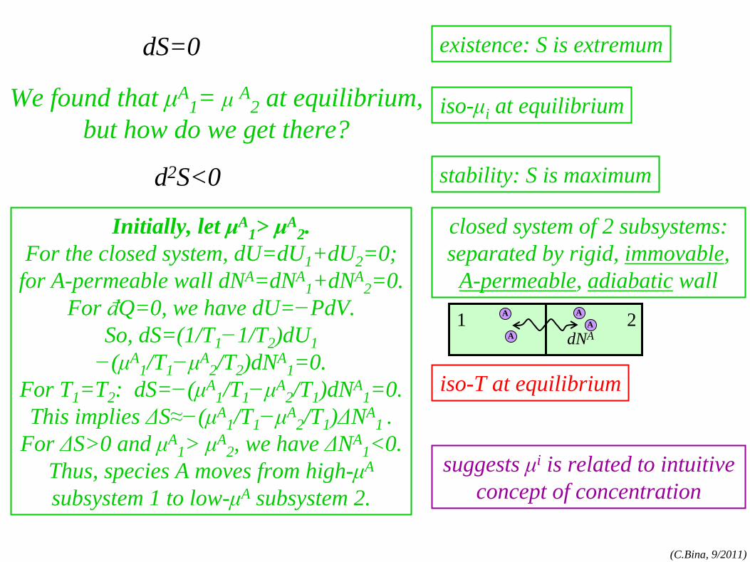
stability: S is maximum
iso-μi at equilibrium
d2S<0
We found that μA1 = μ
A2
at equilibrium,but how do we get there?
existence: S is extremumdS=0
Initially, let μA1 > μA
2 .
For the closed system, dU=dU1 +dU2
=0;for A-permeable wall dNA=dNA
1 +dNA
2 =0.
For đQ=0, we have dU=−PdV.So, dS=(1/T1
−1/T2 )dU1
−(μA1 /T1 −μA
2 /T2
)dNA1 =0.
For T1 =T2
: dS=−(μA1 /T1 −μA
2 /T1
)dNA1 =0.
This implies ΔS≈−(μA1 /T1 −μA
2 /T1
)ΔNA1 .
For ΔS>0 and μA1 > μA
2 , we have ΔNA
1 <0.
Thus, species A moves from high-μA
subsystem 1 to low-μA subsystem 2.
closed system of 2 subsystems: separated by rigid, immovable,
A-permeable, adiabatic wall
suggests μi is related to intuitive concept of concentration
iso-T at equilibrium
1 2dNA
AA
AA
(C.Bina, 9/2011)
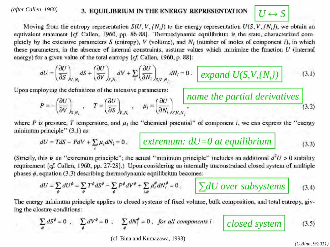
expand U(S,V,{Ni })
U ↔ S
extremum: dU=0 at equilibrium
∑dU over subsystems
closed system
name the partial derivatives
(cf. Bina and Kumazawa, 1993)
(after Callen, 1960)
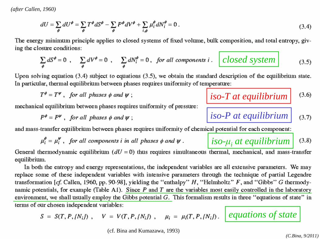
(C.Bina, 9/2011)
closed system
iso-T at equilibrium
iso-P at equilibrium
iso-μi at equilibrium
equations of state(cf. Bina and Kumazawa, 1993)
(after Callen, 1960)
(C.Bina, 9/2011)
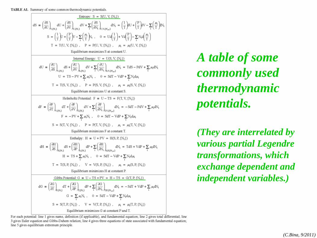
A table of some commonly used thermodynamic potentials.
(They are interrelated by various partial Legendre transformations, which exchange dependent and independent variables.)
(C.Bina, 9/2011)
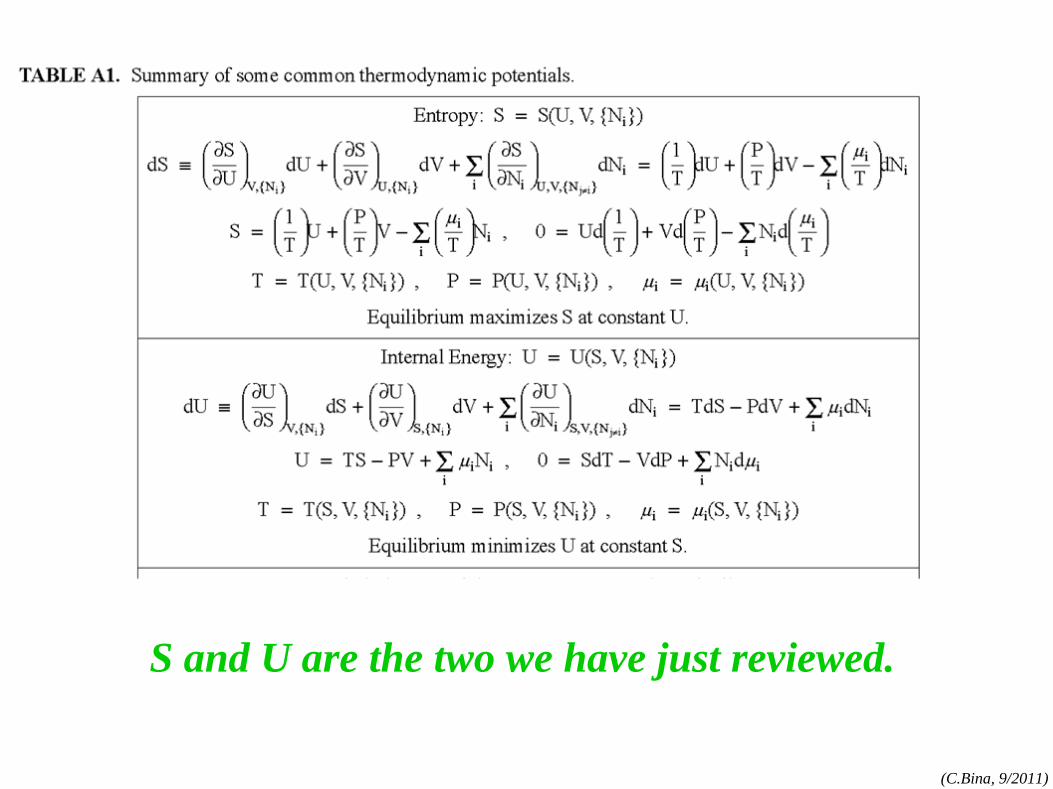
S and U are the two we have just reviewed.
(C.Bina, 9/2011)
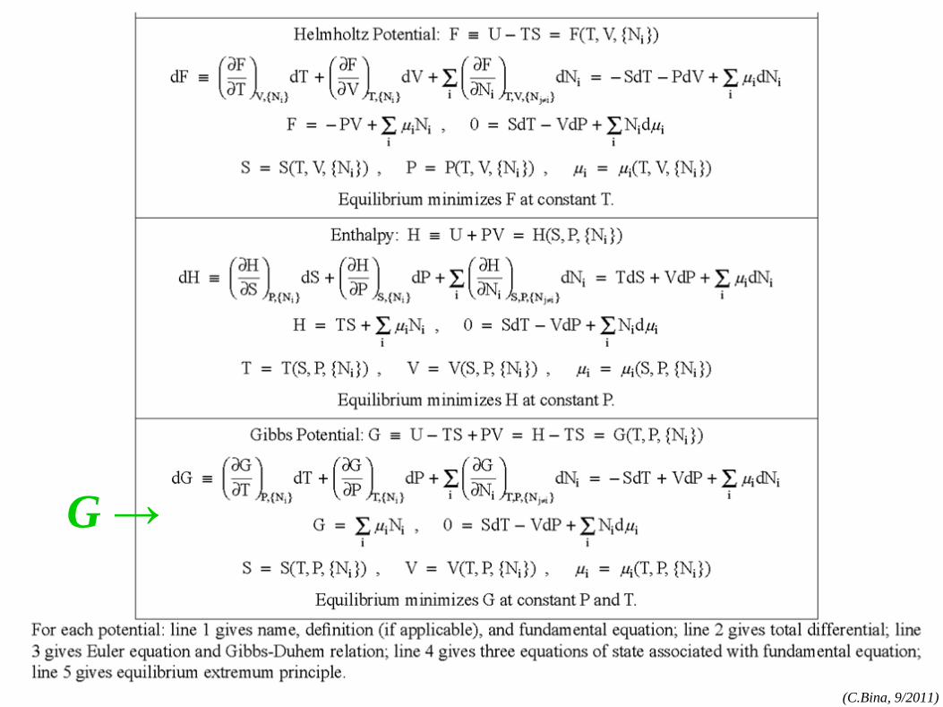
G →
(C.Bina, 9/2011)
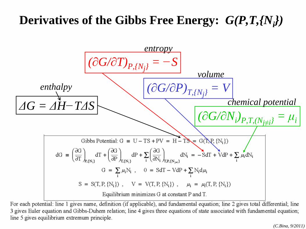
(∂G/∂T)P,{Nj} = −S
(∂G/∂P)T,{Nj} = V
(∂G/∂Ni )P,T,(Nj≠i}
= μi
Derivatives of the Gibbs Free Energy: G(P,T,{Ni })
entropy
volume
chemical potentialΔG = ΔH−TΔSenthalpy
(C.Bina, 9/2011)
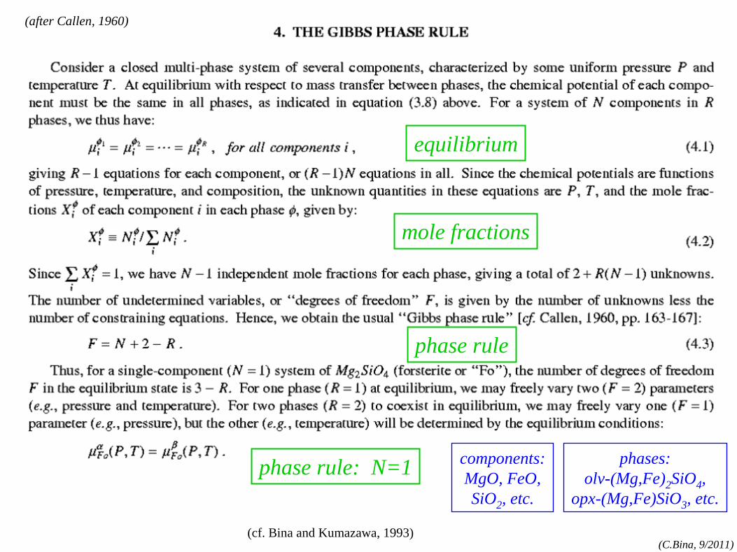
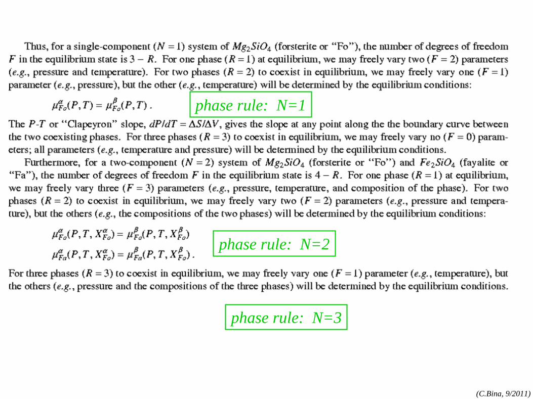
equilibrium
mole fractions
phase rule
phase rule: N=1 components:MgO, FeO,SiO2
, etc.
phases:olv-(Mg,Fe)2
SiO4
,
opx-(Mg,Fe)SiO3 , etc.
(cf. Bina and Kumazawa, 1993)
(after Callen, 1960)
(C.Bina, 9/2011)
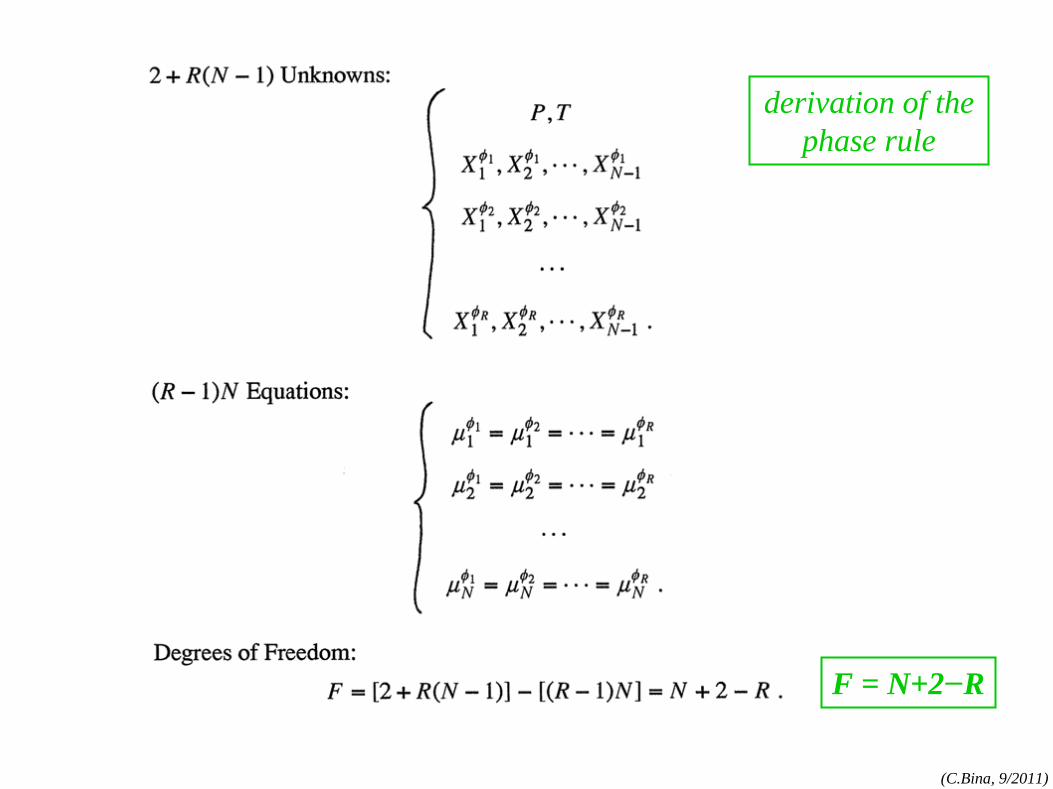
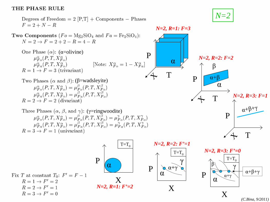
derivation of the phase rule
F = N+2−R
(C.Bina, 9/2011)
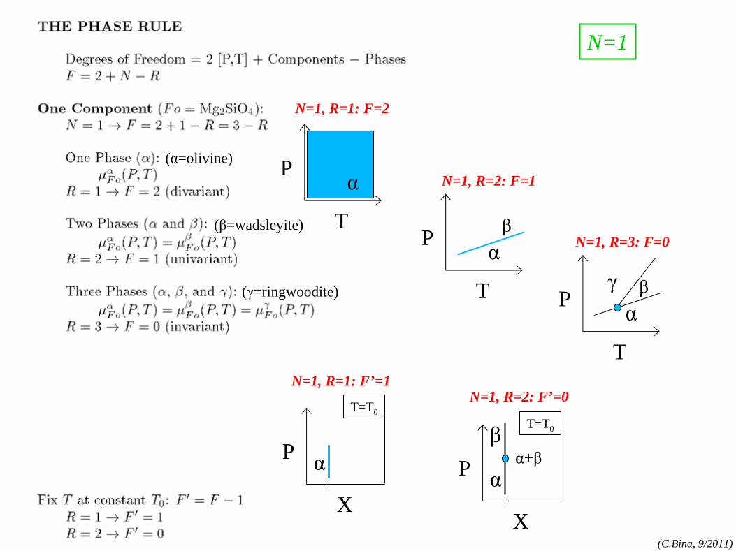
T
P α
T
P αβ
T
P αβγ
X
P
T=T0
αβ
α+β
X
P
T=T0
α
N=1, R=2: F’=0
N=1, R=3: F=0
N=1, R=2: F=1
N=1, R=1: F=2
N=1, R=1: F’=1
N=1
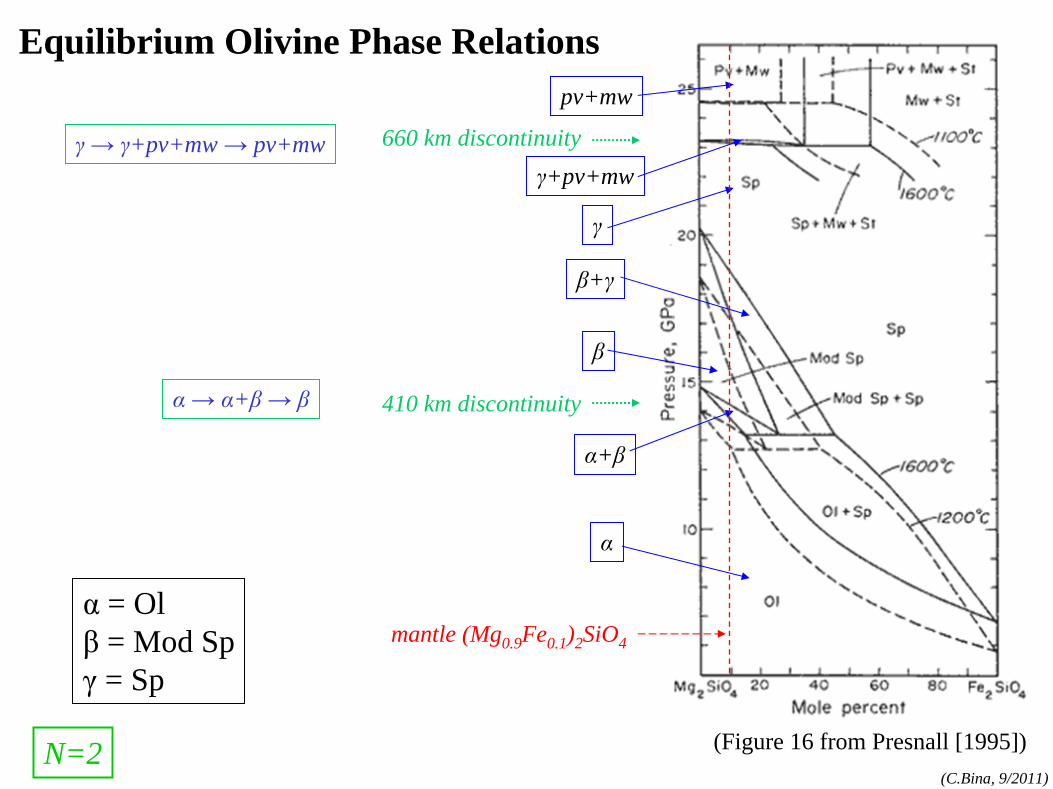
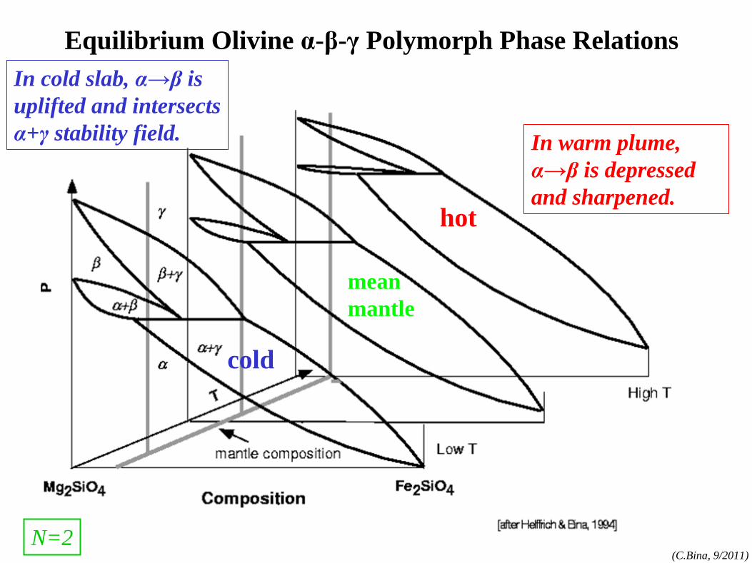
(α=olivine)
(β=wadsleyite)
(γ=ringwoodite)
(C.Bina, 9/2011)
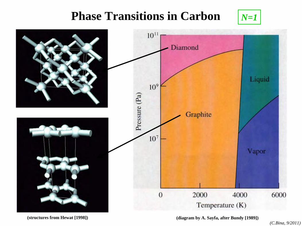
Phase Transitions in Carbon
(diagram by A. Sayfa, after Bundy [1989])(structures from Hewat [1998])