Page 1
VYSOKÉ UČENÍ TECHNICKÉ V BRNĚ BRNO UNIVERSITY OF TECHNOLOGY
FAKULTA PODNIKATELSKÁ ÚSTAV INFORMATIKY
FACULTY PODNIKATELSKÁ DEPARTMENT OF INFORMATICS
PROSTŘEDKY TEORIE HER V EKONOMICKÉM ROZHODOVÁNÍ
TOOLS OF GAME THEORY IN ECONOMIC DECISION MAKING
DIPLOMOVÁ PRÁCE MASTER‘S THESIS
AUTOR PRÁCE Bc. RICHARD ŠEBEDOVSKÝ AUTHOR
VEDOUCÍ PRÁCE prof. RNDr. IVAN MEZNÍK, CSc. SUPERVISOR
BRNO 2012
Page 2
Vysoké učení technické v Brně Akademický rok: 2011/2012Fakulta podnikatelská Ústav informatiky
ZADÁNÍ DIPLOMOVÉ PRÁCE
Šebedovský Richard, Bc.
Informační management (6209T015)
Ředitel ústavu Vám v souladu se zákonem č.111/1998 o vysokých školách, Studijním azkušebním řádem VUT v Brně a Směrnicí děkana pro realizaci bakalářských a magisterskýchstudijních programů zadává diplomovou práci s názvem:
Prostředky teorie her v ekonomickém rozhodování
v anglickém jazyce:
Tools of Game Theory in Economic Decision Making
Pokyny pro vypracování:
ÚvodVymezení problému a cíle práceTeoretická východiska práceAnalýza problému a současná situaceVlastní návrhy řešení, přínos návrhů řešeníZávěrSeznam použité literaturyPřílohy
Podle § 60 zákona č. 121/2000 Sb. (autorský zákon) v platném znění, je tato práce "Školním dílem". Využití této
práce se řídí právním režimem autorského zákona. Citace povoluje Fakulta podnikatelská Vysokého učení
technického v Brně.
Page 3
Seznam odborné literatury:
MAŇAS, Miloslav Teorie her a optimální rozhodování. Praha: SPN,1963 NEUMANN, John, MORGENSTERN, Oskar Theory of Games and Economic Behavior.Princeton: Princeton University Press, 1953 NICHOLSON,Walter Microeconomic Theory. Orlando:The Dryden Press, 1998.ISBN0-03-024474-9NICHOLSON, Walter Intermediate Microeconomics and its Applications. Orlando: The DrydenPress, 2000. ISBN 0-03-025916-9
Vedoucí diplomové práce: prof. RNDr. Ivan Mezník, CSc.
Termín odevzdání diplomové práce je stanoven časovým plánem akademického roku 2011/2012.
L.S.
_______________________________ _______________________________Ing. Jiří Kříž, Ph.D. doc. RNDr. Anna Putnová, Ph.D., MBA
Ředitel ústavu Děkan fakulty
V Brně, dne 23.05.2012
Page 4
Abstrakt
Tato práce se zabývá současnými trendy v aplikaci teorie her k tvorbě ekonomických
modelů, které se následně využívají při ekonomickém rozhodování s podporou
prostředků informatiky. Práce se zejména opírá o poznatky teorie statických
a dynamických her a her s dokonalými a nedokonalými informacemi. Zkoumány jsou
modely týkající se sdílení zdrojů, aukcí a managementu. Pro každý z popsaných modelů
je prezentována konkrétní aplikace.
Abstract
This thesis deals with the present trends in application of game theory to creation of
economic models, which are subsequently used in economic decision making with the
support of tools of information technology. It mainly focuses on the tools of static and
dynamic games and games with perfect and imperfect information. Models of resource
sharing, auctions and management are under investigation. For each of the described
models a concrete application is presented.
Klíčová slova
Teorie her, Nashovo ekvilibrium, Bayesovské Nashovo ekvilibrium, statické hry, dynamické hry, modely oligopolů
Keywords
Game theory, Nash equilibrium, Bayesian Nash equilibrium, static games, dynamic games, Oligopoly models
Page 5
Citace
ŠEBEDOVSKÝ Richard: Tools of game theory in economic decision making, diplomová práce, Brno, FP VUT v Brně, 2012, 82s.
Page 6
Tools of Game theory in economic decision making
Prohlášení
Prohlašuji, že předložená diplomová práce je původní a zpracoval jsem ji samostatně. Prohlašuji, že citace použitých pramenů je úplná, že jsem ve své práci neporušil autorská práva (ve smyslu Zákona č. 121/2000 Sb., o právu autorském a o právech souvisejících s právem autorským). V Brně dne 20. května 2012
…………………… Richard Šebedovský
Page 7
Poděkování
Ďakujem vedúcemu RNDr. Ivanovi Mezníkovi, CSC za odborné vedenie, ochotu, a užitočné pripomienky. © Richard Šebedovský, 2012 Tato práce vznikla jako školní dílo na Vysokém učení technickém v Brně, Fakultě podnikatelské. Práce je chráněna autorským zákonem a její užití bez udělení oprávnění autorem je nezákonné, s výjimkou zákonem definovaných případů.
Page 8
Table of contents Introduction ..................................................................................................................... 10
1 Aim of the work ...................................................................................................... 11
2 Theoretical basis of the work .................................................................................. 12
2.1 Game ................................................................................................................ 12
2.1.1 Static games .............................................................................................. 12
2.1.2 Dynamic games ......................................................................................... 12
2.1.3 Games with incomplete information ......................................................... 12
2.1.4 Cooperative games .................................................................................... 13
2.2 Players .............................................................................................................. 13
2.3 Strategies .......................................................................................................... 13
2.4 Payoffs.............................................................................................................. 13
2.4.1 Zero-sum games and non-zero sum games ............................................... 14
2.5 Normal form ..................................................................................................... 14
3 Problem analysis and current situation ................................................................... 15
3.1 Solving a simple game with one player ........................................................... 15
3.2 Game with two players ..................................................................................... 16
3.3 Important simple game examples ..................................................................... 21
3.3.1 Prisoner’s dilemma ................................................................................... 21
3.3.2 Coordination game/stag hunt .................................................................... 23
3.3.3 Battle of the sexes ..................................................................................... 24
3.3.4 Chicken ..................................................................................................... 25
3.3.5 Ultimatum game ....................................................................................... 27
3.3.6 Dictator game ............................................................................................ 27
3.4 Dynamic games ................................................................................................ 27
3.4.1 Extensive form .......................................................................................... 28
3.4.2 Game tree .................................................................................................. 29
3.4.3 Backwards induction ................................................................................. 31
3.4.4 Threats, promises and credibility .............................................................. 32
3.4.5 Subgame perfect equilibrium .................................................................... 34
4 Proposals of solutions and their contributions ........................................................ 35
4.1 Oligopoly models ............................................................................................. 35
Page 9
4.1.1 Cournot model .......................................................................................... 35
4.1.2 Stackelberg model ..................................................................................... 43
4.1.3 Bertrand model ......................................................................................... 46
4.1.4 Contestable markets .................................................................................. 47
4.1.5 Summary of the oligopoly models ............................................................ 50
4.2 Economic views comparison ............................................................................ 50
4.2.1 Accountant’s point of view ....................................................................... 51
4.2.2 Economist’s point of view ........................................................................ 51
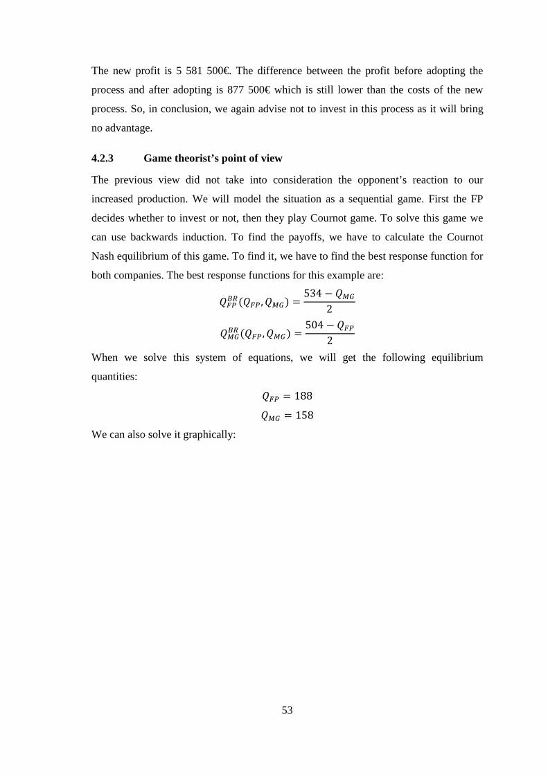
4.2.3 Game theorist’s point of view ................................................................... 53
4.3 Role of uncertainty in decision making ........................................................... 54
4.3.1 Mixed strategies ........................................................................................ 55
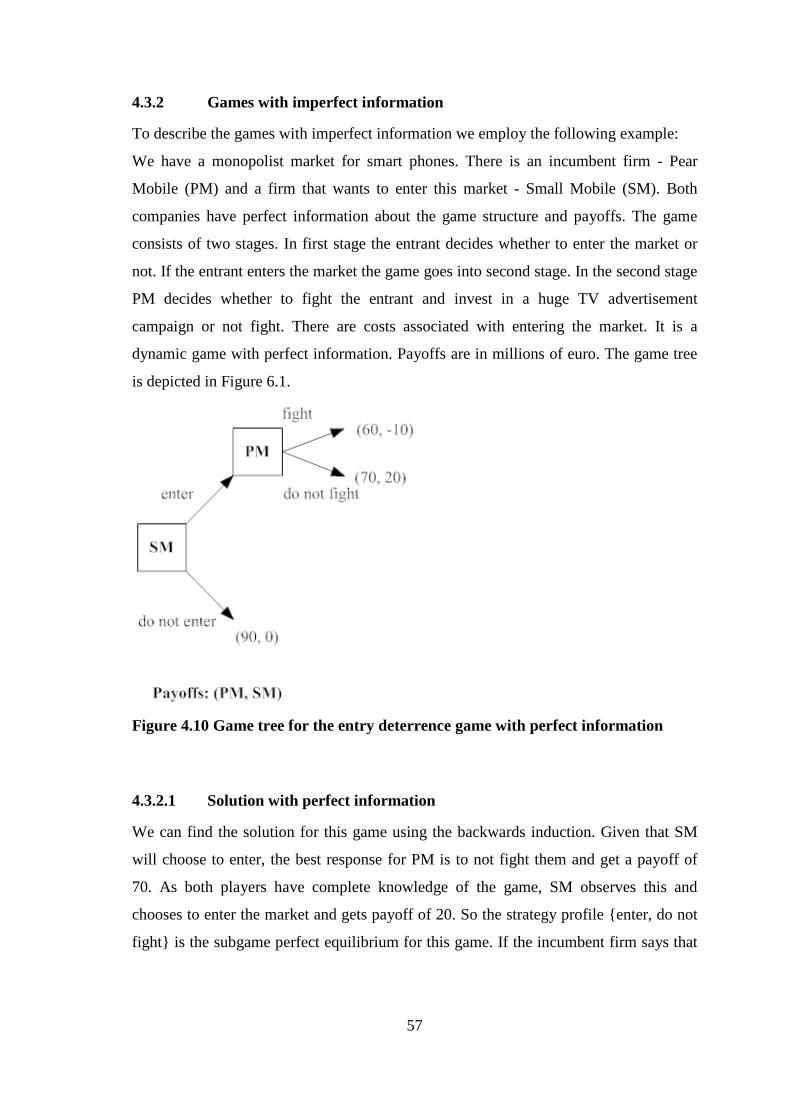
4.3.2 Games with imperfect information ........................................................... 57
4.3.3 Games with incomplete information ......................................................... 60
4.4 Auctions ........................................................................................................... 66
4.4.1 Winner’s curse .......................................................................................... 68
4.4.2 Auction as a game ..................................................................................... 68
4.4.3 Comparison of auction types with perfect information ............................ 68
4.4.4 Comparison of auction types with imperfect information ........................ 72
4.5 Computer science and game theory ................................................................. 74
4.5.1 Languages, libraries and simulation tools ................................................. 74
4.5.2 Routing ...................................................................................................... 74
4.5.3 Online advertisements and auctions ......................................................... 76
4.5.4 Peer-to-peer systems ................................................................................. 76
4.5.5 Other applications ..................................................................................... 77
5 Conclusion .............................................................................................................. 78
6 Bibliography ........................................................................................................... 79
List of Figures ................................................................................................................. 81
List of Tables .................................................................................................................. 82
Page 10
10
Introduction
Imagine a classic childhood game of hide-n-seek. One child from the group is selected
to be “it” and has to count to twenty with eyes closed at the base while the other kids
hide. After counting, his task is to find the others and tag them. Hidden kids have to get
to the base without getting tagged. Each one of them has one important decision to
make – where to hide? Should I hide where I’ve been hidden before, or should I hide
where the person that was “it” didn‘t look before? Should I hide together with my
friend? They have to consider other players’ decisions in order to make their own.
We have played games like these since we were children. What this game has in
common with the games game theory analyzes is the process of making strategic
decisions - decisions that are made in order to achieve a certain goal (win the game)
while taking in consideration other players’ decisions. Game theory analyses these
situations where multiple strategic decision makers interact together - they “play a
game”.
In economic context we can consider bargaining about wage between a potential
employee and employer as a game. Each player has a certain goal - the employee to get
the job with the highest wage possible and employer to get the employee to work for
him for the lowest wage possible. But both of them have to consider the other one when
making an offer, the employer (if he wants the employee) cannot offer a wage that is too
low, as the potential employer might get insulted and leave. Same goes for the potential
employee - he cannot ask for a wage that is too high (if he wants the job). This is a
game in the game theoretic sense.
Other example can be when a firm makes a decision whether to enter a new market.
How will the firms that already are in this market react? Will they try to fight? Will the
incumbent firm (firm that is already on the market) try to take preliminary measures to
keep the potential competitors from entering the market? They are also playing a game.
This work’s aim is to describe the models in game theory that are commonly applied to
economic decision making. First, basic concepts of game theory and then basic games
investigated by game theorists are reviewed. The following chapters describe more
complex models and there is also an example of economic application for each one of
them. A few applications using information technology are also presented.
Page 11
11
1 Aim of the work
This work aims to describe and apply the current game theoretic models and methods
on real world strategic economic decision problems. The first two chapters explain the
most basic concepts and tools needed to solve more complicated situations. The
following chapters describe in detail few of the most important theories together with
their applications on more complex examples.
Page 12
12
2 Theoretical basis of the work
This chapter contains basic concepts of game theory needed for further considerations
and constructions.
2.1 Game
To analyze a game from a game theoretical point of view the game has to be clearly
defined. We have to define rules, players and their available strategies and payoffs for
each one of them. Based on the differences in the criteria above we can distinguish a
number of different types of games.
2.1.1 Static games
Static games are the games which are the easiest to analyze. In static games each one of
the players makes his decision simultaneously with the other players-they do not know
the actions of other players at the point of making the decision. After making the
decision the players are assigned payoffs based on the decisions chosen.
(GIBBONS, 1992, p.1)
A game of rock-paper-scissors can serve as an example for this type of games. Both
players simultaneously choose between rock, paper and scissors and both of them
instantly know who has won.
2.1.2 Dynamic games
In dynamic games, players move in a given order. When they are making their move,
they are aware of actions made by players moving before them (but not necessarily all
the moves). An example of a dynamic game can be the game of chess.
(BIERMAN and FERNANDEZ, 1998, p.121)
2.1.3 Games with incomplete information
Games in which one or both of the players has incomplete information about the
payoffs are called games with incomplete information. An economic example can be a
sale of drilling rights for a parcel. The buyers don’t know if there really is a source of
oil in this place or more precisely they don’t know exactly how rich this source is.
Page 13
13
Another example for this kind of games can be buying a used car. The car salesman
knows the true value of the car he is selling, but the buyer does not. This is also an
example of a game with asymmetric information.
2.1.4 Cooperative games
In cooperative games the players cooperate together to achieve their individual goals.
The key in analyzing these games is to find the players’ motivation to cooperate.
Usually it is not simple to model cooperation - see Prisoner’s dilemma in the next
chapter.
2.2 Players
Players are the strategic decision makers in our games. In the wage-bargaining example
in the introduction the players were the employee and the employer. Important notion is
that the players are always considered rational – they always try to take actions which
lead to the best results for them (they are selfish).
2.3 Strategies
A strategy in game theory represents a plan of response to each one of the courses the
game can take. Strategy is a complete plan of actions for the game for the player. A list
of strategies, one for each player, is called a strategy profile.
(BIERMAN and FERNANDEZ, 1998, p.7)
We can distinguish two kinds of strategies based on the presence of random factor:
• Pure strategies - they are not random
• Mixed strategies - they involve a probability for each move
Strategies will be capitalized - for example Buy, Don’t buy. Strategy profiles will be
written in curly braces – {Buy, Don’t buy}, where Buy is the strategy for the first player
and Don’t buy is the strategy for the second player.
2.4 Payoffs
Payoff is the outcome that the player gets for each of the strategy profiles. They
represent what the player gets at the end of the game. In this work the payoffs will be
usually given in terms of monetary gains/losses. In real world people usually consider
Page 14
14
more than just monetary gains. List of payoffs for each strategy profile is called the
payoff vector. Payoffs for simple non-cooperative games can be represented using a
matrix, for example the payoff matrix for the rock-paper-scissors game is depicted in
table 2.1.
Rock Paper ScissorsRock (0, 0) (-1, 1) (1, -1)Paper (1, -1) (0, 0) (-1, 1)Scissors (-1, 1) (1, -1) (0, 0)
Player 2
Player 1
Payoffs: (Player 1, Player 2)
Table 2.1 Payoffs for the rock-paper-scissors game
Where payoff (0, 0) means that both players don’t get anything – it’s a draw, (1, -1)
means that the first player has won and gets a payoff of 1 (1€ for example), (-1, 1)
means that the second player has won and gets a payoff of 1.
2.4.1 Zero-sum games and non-zero sum games
A zero-sum game is the game where what one player loses, the other one wins. In other
words the sum of the payoffs of all players is zero. On the other hand, games where the
sum of payoffs is a non-zero value are called non-zero sum games.
2.5 Normal form
The normal-form representation of a n-player game specifies the players’ strategy
profiles S1,…,Sn and their payoff vectors u1,…,un. We can denote this game by G =
{S1,…,Sn;u1,…, un}.
(GIBBONS, 1992, p.4)
Normal form representation can be used to describe a static game. It is also called the
strategic form of the game.
Page 15
15
3 Problem analysis and current situation
This chapter describes some of the classic games and explains how to solve them. These
games and tools used to solve them will serve as a basis to understand and solve more
complex games in the following chapters. Most important concepts introduced in this
chapter are – game matrix, Nash equilibrium and Focal point equilibrium (Schelling
point).
3.1 Solving a simple game with one player
In this subchapter, a simplified example game will be used to help explain the necessary
tools needed to solve the following games. The game goes as follows:
We have a mid-sized lake in the mountains. In this lake a special kind of pearls of
superb quality was found. These pearls do not regenerate, and it is assumed that there
are 4000 of them in the lake. Each one of the pearls is worth 500€.
The Pearl Hunters company has an exclusive pearl hunting 4-year license for this lake.
The price of pearls does not change over the course of these 4 years. The company has
to make a decision whether to buy a special robot which can search for the pearls.
Without it, using only trained divers, they can expect to find 1000 pearls per year, so
they will find all of the pearls in 4 years. If they buy the robot, they can expect that they
will find 4000 pearls per year, which means they will find all of them in one year. This
special robot costs 750 000€, while the training costs for divers are only 400 000€. The
cost to extract the pearls is 100€ per pearl. The following table sums the expected costs
and revenues.
Divers RobotSearching cost 400 000€ 750 000€Extracting cost 400 000€ 400 000€Total cost 800 000€ 1 150 000€Revenue 2 000 000€ 2 000 000€Profit 1 200 000€ 850 000€ Table 3.1 Sum of costs, revenues and profits for the Pearl Hunters company
Page 16
16
The player in this game is the Pearl Hunters company, its strategy is either to use the
Divers or to use the Robot and the payoffs are respectively 1 200 000€ and 850 000€.
In this example we can say without the use of any additional tools that the most
profitable strategy is to not buy the Robot and use the Divers, getting the payoff of
1 200 000€.
3.2 Game with two players
Now, we will consider one important modification to the previous game. The Pearl
Hunters company does not have an exclusive license for the pearl hunting for the lake.
There is another company that wants to invest in pearl hunting in this lake – Pearl
Seekers. This company is in every aspect the same as the Pearl Hunters. But now there
is one important difference in profits, which are split between the two companies. Both
of the companies share the resources - pearls in the lake. In this game we assume that
money in the future has the same value for the company as money today.
Now we have two players – Pearl Hunters and Pearl Seekers, both of them have two
available strategies –Divers and Robot. So now we have four available strategy profiles:
• {Divers, Divers} – both companies use the Divers strategy
• {Divers, Robot} – Pearl Hunters company uses the Divers strategy, and
the Pearl Seekers company uses the Robot strategy
• {Robot, Divers} – Pearl Hunters company uses the Robot strategy , and
the Pearl Seekers company uses the Divers strategy
• {Robot, Robot} – both companies use the Robot strategy
Each one of the strategy profiles leads to a unique payoff. The payoffs for each strategy
profile can be found in the following table.
Divers RobotDivers (400 000€, 400 000€) (-30 000€, 480 000€)Robot (480 000€, -30 000€) (50 000€, 50 000€)
Pearl Seekers
Pearl Hunters
Payoffs: (Pearl Hunters, Pearl Seekers)
Table 3.2 Payoff matrix for the Pearl Hunters and Pearl Seekers companies
Page 17
17
The players in this game make their decisions simultaneously without knowing the
decision of the other player - it is a static game. Now we will try to find the best
decision that each player can make.
First we will analyze the situation from the Pearl Hunters’ point of view. They do not
know the decision the Pearl Seekers make, but they have to take it into account. If Pearl
Hunters believe that Pearl Seekers will play the Robot strategy than it is reasonable to
also play the Robot strategy, because it yields the payoff of 50 000€, compared to a
payoff of -30 000€ if they would play the Divers strategy. On the other hand if Pearl
Hunters believe that Pearl Seekers will play the Divers strategy, than the best they can
do is to play the Robot strategy again and get a payoff of 480 000€, compared to payoff
of 400 000€. So we can say that playing the Robot strategy strictly dominates playing
the Divers strategy, or that the Divers strategy is strictly dominated by the Robot
strategy. It means that it is never rational to play the Divers strategy in this game.
Formally:
“The strategy S1 strictly dominates the strategy S2 for a player if, given any collection
of strategies, that could be played by the other players, playing S1 results in a strictly
higher payoff for that player than does playing S2. The strategy S2 is also said to be
strictly dominated by S1. A rational player will never adopt a strictly dominated
strategy nor expect a rational opponent to adopt one.”
(BIERMAN and FERNANDEZ, 1998, p.9)
At this point we can start looking for strictly dominated strategies in our game and
eliminate them. We can eliminate the Divers strategy, as this one will never be played.
This leaves us with only one strategy left - Robot. This strategy is strictly dominant.
“A strictly dominant strategy for a player is one that strictly dominates every other
strategy of that player. A rational player will adopt a strictly dominant strategy
whenever it exists”.
(BIERMAN and FERNANDEZ, 1998, p.10)
Because our players’ payoffs are symmetrical, we now know that Pearl Seekers will
also play the Robot strategy. We have only one strategy left for each player. The game
is solved. The solution is a strictly dominant strategy equilibrium.
Page 18
18
“The strategy profile (S1,…,Sn) is a strictly dominant strategy equilibrium if for
every player i, Si is a strictly dominant strategy”.
(BIERMAN and FERNANDEZ, 1998, p.10)
But this equilibrium solution has one problem. The players are much worse off playing
these equilibrium strategies than if they both play the Divers strategy. If both players
can cooperate and play the Divers strategy they can both have payoffs of 400 000€ -
350 000€ more than when both playing the Robot strategy. The equilibrium outcome is
Pareto dominated.
“The outcome O of a game is Pareto dominated if there is some other outcome O’ such
that:
(1) every player either strictly prefers O’ to O or is indifferent between O’ and O,
and
(2) some player strictly prefers O’ to O.
An outcome is Pareto optimal if it is not Pareto dominated by any other outcome of the
game”.
(BIERMAN and FERNANDEZ, 1998, p.12)
To give a more complete list of basic definitions we will also define weak dominance:
“The strategy S1 weakly dominates the strategy S2 for a player if, given any collection
of strategies that could be played by the other players, playing S1 never results in a
lower payoff to that player than does playing S2 and, in at least one instance, S1 gives
the player a strictly higher payoff than does S2. The strategy S2 is said to be weakly
dominated by S1. A rational player will seldom play a weakly dominated strategy.
A weakly dominant strategy for a player is one that weakly dominates every other
strategy of that player. A rational player will usually play a weakly dominant strategy.
The strategy profile (S1, S2,…, Sn) is a weakly dominant strategy equilibrium if for
every player i, Si is a weakly dominant strategy”.
(BIERMAN and FERNANDEZ, 1998, p.12)
If we slightly modify the previous game and add the option to use neither Divers nor the
Robot we will get a different payoff scheme:
Page 19
19
Divers Robot NothingDivers (400 000€, 400 000€) (-30 000€, 480 000€) (1 200 000€, 0€)Robot (480 000€, -30 000€) (50 000€, 50 000€) (850 000€, 0€)Nothing (0€, 1 200 000€) (0€, 850 000€) (0€, 0€)
Pearl Hunters
Pearl Seekers
Payoffs: (Pearl Hunters, Pearl Seekers)
Table 3.3 Payoffs for the pearl-hunting game with 3 strategies
In this modified game dominant strategy (weak or strong) no longer exists. Robot
dominates Nothing, but it no longer dominates Divers. Divers and Nothing do not
dominate any other strategy. But from the payoffs it’s easy to see that the Nothing
strategy will never be used, as the players can guarantee themselves at least the outcome
of using Robot, which is at least 50 000€, which is better than 0€. The Nothing strategy
is strictly dominated so we can eliminate it. When we eliminate the Nothing strategy we
are left with the same result as before – to play the Robot strategy. This strategy is
called iterated strictly dominant.
“A strategy is iterated strictly dominant for player i if and only if it is the only strategy
in -Si, where -Si is the intersection of the following sequence of nested sets of strategies:
(1) Si1 consists of all of player i’s strategies that are not strictly dominated
(2) For n > 1, Sin consists of the strategies in Sin-1 that are not strictly dominated
when we restrict the other players j ≠ i to the strategies in Sjn-1.
The strategy profile (S1,S2, …,Sn) is an iterated strictly dominant strategy
equilibrium if for every player i, Si is an iterated strictly dominant strategy”.
(BIERMAN and FERNANDEZ, 1998, p.14)
Iterated weakly dominance is a bit more complicated and will not be used in this
work.
In our example we needed just one iteration to remove the Nothing strategy. In more
complex games, there can be much more iterations.
In most of the games there will be more than one iterated strategy equilibrium. Example
for such a game can be a modified pearl hunting game. The payoff scheme of this
modified game is shown in table 3.4.
Page 20
20
Divers Robot NothingDivers (400 000€, 400 000€) (60 000€, 480 000€) (1 200 000€, 0€)Robot (480 000€, 60 000€) (50 000€, 50 000€) (850 000€, 0€)Nothing (0€, 1 200 000€) (0€, 850 000€) (0€, 0€)
Pearl Seekers
Pearl Hunters
Payoffs: (Pearl Hunters, Pearl Seekers)
Table 3.4 Payoffs for the modified pearl-hunting game with 3 strategies
The difference is that when one of the companies uses the Divers strategy and the other
one uses the Robot, they now don’t get a loss of 30 000€, but instead they make a profit
of 60 000€.
Again, the Nothing strategy is strictly dominated for both Pearl Hunters and Pearl
Seekers, as both firms can make more than 0€ in all cases using either the Divers or
Robot strategy. So the Nothing strategy can be eliminated. The following table shows
the payoff scheme after the elimination of dominated strategy.
Divers RobotDivers (400 000€, 400 000€) (60 000€, 480 000€)Robot (480 000€, 60 000€) (50 000€, 50 000€)
Pearl Seekers
Pearl Hunters
Payoffs: (Pearl Hunters, Pearl Seekers)
Table 3.5 Payoffs for the modified pearl-hunting game with 3 strategies without the dominated strategies
Now there are no dominated strategies to eliminate. Both of the players are assumed to
be rational, so they will always play the strategy which has the best outcome for them.
If Pearl Hunters believe that Pearl Seekers will use Robot, then they have two options:
• Use Robot too and earn 50 000€
• Use Divers and earn 60 000€
The rational choice for Pearl Hunters is to use Divers (play the Divers strategy) and earn
60 000€. The Divers strategy is the best response to the Robot strategy being played by
Page 21
21
Pearl Seekers. Now if Pearl Seekers believe that Pearl Hunters will use Divers they have
two options too:
• Use Divers too and earn 400 000€
• Use Robot and earn 480 000€
The rational choice for Pearl Seekers now is to use Robot and earn 480 000€, which is a
best response to the Divers strategy being played by the Pearl Hunters. The result is that
players will adopt the strategy profile {Robot, Divers}. This belief is self-confirming,
meaning that it is the rational choice for both players and neither one of them can do
any better by unilaterally changing their choice. Because the payoff scheme is
symmetrical, the same is true for the strategy profile {Divers, Robot}. This is the
concept of the Nash equilibrium named after Professor John C. Nash. The formal
definition is:
“Suppose there are N players in a game, Xi is the set of possible strategies for player i,
and vi(s1, …, sN) is player i’s payoff when the players choose the strategy profile {si, …,
sN}. A Nash equilibrium is a strategy profile {si*, sN
*} such that each strategy si* is an
element of Xi, and maximizes the function fi(x) = vi(si*, …, si-1
*, x, si+1*, …, sN
*) among
the elements of Xi. That is, at a Nash equilibrium, each player’s equilibrium strategy is a
best response to the belief that the other players will adopt their Nash equilibrium
strategies”.
(BIERMAN and FERNANDEZ, 1998, p.16)
3.3 Important simple game examples
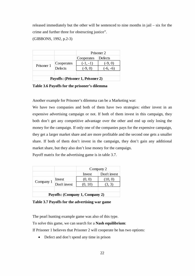
3.3.1 Prisoner’s dilemma
Prisoner’s dilemma is a classic game whose result is not Pareto optimal.
The story goes:
“Two suspects are arrested and charged with a crime. The police lack sufficient
evidence to convict the suspects, unless at least one confesses. The police hold the
suspects in separate cells and explain the consequences that will follow from the actions
they could take. If neither confesses then both will be convicted of a minor offense and
sentenced to a one month in jail. If both confess then both will be sentenced to jail for
six months. Finally, if one confesses but the other does not, then the confessor will be
Page 22
22
released immediately but the other will be sentenced to nine months in jail – six for the
crime and further three for obstructing justice”.
(GIBBONS, 1992, p.2-3)
Cooperates DefectsCooperates (-1, -1) (-9, 0)Defects (-9, 0) (-6, -6)
Payoffs: (Prisoner 1, Prisoner 2)
Prisoner 1
Prisoner 2
Table 3.6 Payoffs for the prisoner’s dilemma
Another example for Prisoner’s dilemma can be a Marketing war:
We have two companies and both of them have two strategies: either invest in an
expensive advertising campaign or not. If both of them invest in this campaign, they
both don’t get any competitive advantage over the other and end up only losing the
money for the campaign. If only one of the companies pays for the expensive campaign,
they get a larger market share and are more profitable and the second one gets a smaller
share. If both of them don’t invest in the campaign, they don’t gain any additional
market share, but they also don’t lose money for the campaign.
Payoff matrix for the advertising game is in table 3.7.
Invest Don't investInvest (0, 0) (10, 0)Don't invest (0, 10) (3, 3)
Company 2
Company 1
Payoffs: (Company 1, Company 2) Table 3.7 Payoffs for the advertising war game
The pearl hunting example game was also of this type.
To solve this game, we can search for a Nash equilibrium:
If Prisoner 1 believes that Prisoner 2 will cooperate he has two options:
• Defect and don’t spend any time in prison
Page 23
23
• Cooperate and spend a month in prison
The rational choice is to defect and not go to jail. Now if Prisoner 2 believes that
Prisoner 1 will defect, he has two options:
• Defect and get 6 months in prison
• Cooperate and get 9 months in prison
His best response is to defect, so strategy profile {Defect, Cooperate} is not a Nash
equilibrium and neither is {Cooperate, Cooperate}.
Now suppose that Prisoner 1 believes that Prisoner 2 will defect. He has two options:
• Defect and get 6 months in prison
• Cooperate and get 9 months in prison
Rationally he will choose to defect and because the payoffs in the game are
symmetrical, Player 2 will defect too. In conclusion, there is only one Nash equilibrium
in this game, the strategy profile {Defect, Defect} – both players will defect and spend 6
months in jail (both will invest in the ad campaign and make zero profit). This outcome
is Pareto dominated by the {Cooperate, Cooperate} strategy profile’s outcome, which is
one of the reasons why is Prisoner’s dilemma one of the most known and studied game
of game theory.
3.3.2 Coordination game/stag hunt
The coordination game goes like this:
You want to go on a date with your girlfriend to a classy restaurant. Your girlfriend
prefers going to this restaurant dressed in formal clothing. You feel the same way. Most
important is that both of you go to the restaurant dressed the same way.
The payoffs are represented in the following table.
Formal CasualFormal (2, 2) (0, 0)Casual (0, 0) (1, 1)
Your girlfriend
You
Payoffs: (You, Your girlfriend)
Table 3.8 Payoffs for the coordination game
Page 24
24
This game is usually called the coordination game, as both players have to coordinate
their moves to get the best result. In this instance it is going to the restaurant formally
dressed.
Another variant of this game is called the stag hunt:
Two hunters go on a hunt. They both have two options:
• Hunt a stag
• Hunt a hare
They both make their decisions simultaneously and independently of each other. If they
want to hunt the stag, they need to cooperate. They can hunt a hare alone, but the hare is
worth less than a stag. The payoff scheme is the same as in the previous example.
There are two Nash equilibria:
• Both dress formally/Both go stag hunting
• Both dress casually/Both go hare hunting
But for the players to choose the Pareto optimal one – Formal/Stag we have to make a
few assumptions about the game. We have to assume that:
• Both players know the payoff scheme – it is common knowledge
• Both players are rational – they try to maximize their payoffs given their
knowledge about the game
• Both players prefer formal to casual/stag to hare
3.3.3 Battle of the sexes
This game is similar to the coordination game, but there is a slight modification. This
time you want to go on a date with your girlfriend to a medium-class restaurant. Your
girlfriend prefers going to this restaurant dressed in formal clothing. But you prefer
going there dressed casually. But again, both of you prefer going to the restaurant
dressed the same way to dressing differently.
The payoffs are represented in the following table.
Page 25
25
Formal CasualFormal (1, 2) (0, 0)Casual (0, 0) (2, 1)
Your girlfriend
You
Payoffs: (You, Your girlfriend)
Table 3.9 Payoffs for the Battle of the sexes game
This game is usually called the Battle of the sexes. There are two Nash equilibria in this
game: {Formal, Casual} and {Casual, Formal}. Without using threats/promises or
changing the game there is no single solution to this game (no way to select one of the
Nash equilibria), because any kind of reasoning that leads you to choose Casual
clothing will lead your girlfriend to choose Formal, leading to the payoff scheme (0, 0).
Another way of solving the problem is to use the concept of focal point (or Schelling
point), introduced by Thomas Schelling. A focal point is a Nash equilibrium (in games
that have them) that somehow stands out as the best solution. As Schelling states it:
“Most situations -- perhaps every situation for people who are practiced at this kind of
game -- provide some clue for coordinating behavior, some focal point for each
person’s expectation of what the other expects him to expect to be expected to do.
Finding the key, or rather finding a key -- any key that is mutually recognized as the
key becomes the key -- may depend on imagination more than on logic; it may depend
on analogy, precedent, accidental arrangement, symmetry, aesthetic or geometric
configuration, casuistic reasoning, and who the parties are and what they know about
each other”.
(SCHELLING, 1970, p.57)
An example of a focal point can be:
You have been to a few dates with your girlfriend and she always dresses formally. So it
is safe to assume that she will do it this time again and you should do the same. So the
strategy profile {Formal, Formal} is a Schelling point in this example.
3.3.4 Chicken
The game goes like this:
Page 26
26
There are two drivers going against each other on a narrow road – you and your
opponent. The one that swerves is called the chicken. There are four possible outcomes
for this game:
• The opponent swerves, he is the chicken, you are the winner
• You swerve, you are the chicken, he is the winner
• Both of you swerve, both of you are chickens
• None of you swerve, cars crash, both of you are dead
The payoffs can be represented with the following table:
Don't swerve SwerveDon't swerve (-5, -5) (2, -1)Swerve (-1, 2) (0, 0)
The opponent
You
Payoffs: (You, Your opponent)
Table 3.10 Payoffs for the game of Chicken
There can be many variants for this game, for example:
A company has got into problems. The unionized workers are demanding salary raises,
threatening they will go on a strike. If the management gives in to their demands, it
loses its power (and money). If the workers give up, the union loses its power (and also
money). If they both give in, nobody gains anything. But if both sides refuse to give in,
there will be a strike, which is the worst outcome for both sides (same as crash in the
previous example).
The Nash equilibria in this example are the ones where one of the players swerves/gives
in and the other one does not. The profile {Swerve, Swerve} is not a Nash equilibrium,
because if any of the players knew that the other one is going to swerve, he will choose
not to swerve and “win” the game. But there is no simple way to decide which Nash
equilibrium will actually be played. One way to solve these games is again the Schelling
point (if the management has given in a few times before, it is reasonable they will do it
again).
Page 27
27
3.3.5 Ultimatum game
This game has been practically studied by many game theorists, economists and
psychologists. It is usually stated like this:
Player A is given a sum of money. He has to offer Player B a portion of this money. If
Player B accepts his proposal, they split the money according to the proposal. But if
Player B rejects the offer, both of them get nothing. Therefore Player A makes an
ultimatum.
The classic game theoretic solution is that Player B should and will accept any offer, as
any monetary gain is preferred to none. So Player A should make the minimal offer
possible and this offer will be accepted. This game has been modified and practically
played in many ways, but most of the time, the game theoretic solution was in reality
not used, as minimal offers were rejected by Player B. There are various explanations
for that using the knowledge of psychology, sociology or the concepts of evolutionary
game theory.
(BEARDEN, 2001)
3.3.6 Dictator game
The dictator game is a variation of the ultimatum game. The game goes as follows:
Player A is given a sum of money and he has to propose a split with player B. Player B
is then given his portion and player A keeps the rest.
This is not exactly an example of a game, but it is a case of strategic decision of one
player (it is a degenerate game). The game theoretic solution in this case is to offer
Player B nothing and keep all the money. But in the experiments, again this solution
was not used. Majority of the results showed that Player A proposed a non-zero sum of
money to Player B, displaying altruism. It proves that players in real life consider not
only monetary gains.
(BEARDEN, 2001)
3.4 Dynamic games
In dynamic games the players do not make their decisions at the same time, but they do
it in a given sequence. The order of moves affects the solutions for these games,
Page 28
28
because the players moving later in the game observe the moves made before and make
their decisions considering that.
3.4.1 Extensive form
To completely describe a dynamic game, we can use its extensive form. The extensive
form consists of:
1. Set of players – a list of players playing the game. One special player is Nature –
it represents exogenous actions. Nature does not play a role in every game.
Nature’s moves are usually associated with external events that happen with
some probability.
2. Order of events – this order is usually described by the game tree. It describes
the possibilities each player has at certain points in the game. The game tree has
to have a unique initial node, the root, from which the game begins. A finite
path of predecessors from each node of the tree to the root has to exist. Each
node is immediately preceded by only one node (except from the root). Each
path of the game has to reach a terminal node. The path to the terminal node
represents the individual decisions that had to be made to get to that terminal
node – the game history.
3. Order of moves – each node has a player assigned to them. Nature, if present,
moves first and determines the outcome.
4. Available actions – at each node the player whose order it is to play has a set of
available actions. The number of actions is equal to the number of nodes that
immediately success the current node. Each successor is associated with one
unique action.
5. Information sets – Information sets are used to model games of imperfect
information. When certain nodes are grouped into information sets, the player
cannot distinguish at which node he really is – he does not know what the
preceding decisions were. The available actions have to be the same for all of
the nodes in one information set (otherwise the player can actually distinguish
the nodes).
6. Payoffs – each terminal node is associated with a certain payoff for each player.
Nature does not have payoffs.
(VEGA-REDONDO, 2003)
Page 29
29
I will explain the necessary tools needed to solve dynamic games on the following
example:
Two influential political parties are arguing about two new laws that are going to be
voted in the parliament. The law that is going to be voted for the first is the new
Commercial code, which is going to change the way the minimum wage is calculated –
effectively it is going to get higher. The Labour party is a supporter of this law. The
second law legalizes same-sex marriage. The Liberal party is a supporter of this law.
Liberal party does not really care about the Commercial code law, and the Labour party
does not care about the same-sex marriages law. But it is of value if they vote the same
(to show the public that they stand together). Neither of the parties alone has the power
to push the law they want, but together they have enough members to push the vote. It is
known that the Labour party is going to vote for the Commercial code and the Liberal
party for the same-sex marriages. The Labour party will know if the Liberal party voted
for or against the Commercial code before the same-sex marriages law is going to be
voted. Both parties know before what is the stance of the other party on these laws – it
is a game of perfect information.
3.4.2 Game tree
The resulting sequential game can be illustrated using a special kind of graph - a game
tree:
Figure 3.1 Game tree for the politics game
Page 30
30
The nodes in the tree represent the points where the parties have to make their
decisions. Both players know the previous decisions. The outcomes of the game can be
also represented using a table:
• CC+/CC- means for/against the Commercial code
• SSM+/SSM- means for/against the same-sex marriages
CC+ CC-SSM+ (5, 5) (4, -1)SSM- (0, 4) (1, 1)
Liberal
Labour
Payoffs: (Liberal, Labour)
Table 3.11 Payoffs for the politics game
First we can find the Nash equilibria in this game using the strategic form of this game.
The strategic form shows the payoffs for each strategy profile:
CC+ CC-(SSM+, SSM+) (5, 5) (4, -1)(SSM+, SSM-) (5, 5) (1, 1)(SSM-, SSM+) (0, 4) (4, -1)(SSM-, SSM-) (0, 4) (1, 1)
Liberal
Labour
Payoffs: (Liberal, Labour)
Table 3.12 Strategic form of the politics game
From the strategic form of the game we can try to find the Nash equilibria by evaluating
each strategy profile.
• If the Labour party plays (SSM+, SSM+) strategy, then Liberal party will choose
to play CC+. If the Liberal plays CC+, then the Labor party cannot do better
than play (SSM+, SSM+), so {CC+, (SSM+, SSM+)} is a Nash equilibrium.
Page 31
31
• If the Labour party plays (SSM+, SSM-), then Liberals are better of playing
CC+. If the Liberal party plays CC+, then the Labor party cannot do better than
play (SSM+, SSM-) , so {CC+, (SSM+, SSM-)} is a Nash equilibrium.
• If the Labour party plays (SSM-, SSM+), then Liberals are better off playing
CC-. If the Liberal party plays CC-, then playing (SSM+, SSM+) is better than
playing (SSM-, SSM+), so it is not a Nash equilibrium.
• If the Labour party plays (SSM-, SSM-), then Liberals are better of playing CC-.
If the Liberal party plays CC-, then Labour party cannot do better than play
(SSM-, SSM-), so {CC-, (SSM-, SSM-)} is a Nash equilibrium.
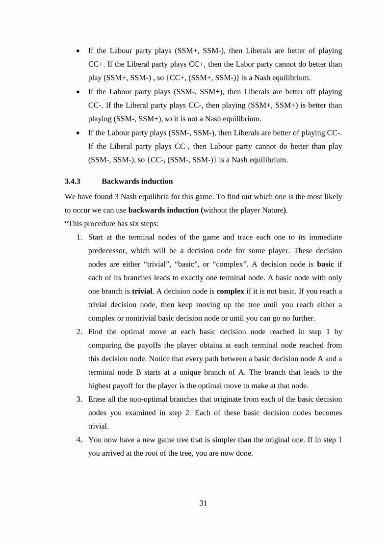
3.4.3 Backwards induction
We have found 3 Nash equilibria for this game. To find out which one is the most likely
to occur we can use backwards induction (without the player Nature).
“This procedure has six steps:
1. Start at the terminal nodes of the game and trace each one to its immediate
predecessor, which will be a decision node for some player. These decision
nodes are either “trivial”, “basic”, or “complex”. A decision node is basic if
each of its branches leads to exactly one terminal node. A basic node with only
one branch is trivial. A decision node is complex if it is not basic. If you reach a
trivial decision node, then keep moving up the tree until you reach either a
complex or nontrivial basic decision node or until you can go no further.
2. Find the optimal move at each basic decision node reached in step 1 by
comparing the payoffs the player obtains at each terminal node reached from
this decision node. Notice that every path between a basic decision node A and a
terminal node B starts at a unique branch of A. The branch that leads to the
highest payoff for the player is the optimal move to make at that node.
3. Erase all the non-optimal branches that originate from each of the basic decision
nodes you examined in step 2. Each of these basic decision nodes becomes
trivial.
4. You now have a new game tree that is simpler than the original one. If in step 1
you arrived at the root of the tree, you are now done.
Page 32
32
5. If you have not yet reached the root, then go back to step 1 and start all over
again. In this way, you work your way step by step toward the root.
6. For each player, collect together the optimal decisions at each of the player’s
decision nodes. This collection of decisions constitutes that player’s optimal
strategy in the game.”
(BIERMAN and FERNANDEZ, 1998, p.129-130)
Now we can apply this rule to the previous example.
First we find the optimal decision of the Labour party at the bottom decision node. If
they support SSM, they get a payoff of -1, if they do not support, they get a payoff of
+1, so the optimal decision is to not support SSM. In the upper node the optimal
solution is to support SSM and get a payoff of 5 compared to 4 when voting against
SSM. After eliminating the non-optimal branches the game tree looks as depicted in
figure 3.3.
Figure 3.2 Game tree after elimination of non-optimal branches
The only thing left is to find the optimal decision for the Liberal party at the remaining
node. The optimal decision is to support the CC and get a payoff of 5 compared to not
supporting and payoff of 1. So the only Nash equilibrium strategy profile left after the
backwards induction is applied is {CC+, (SSM+, SSM-)}.
3.4.4 Threats, promises and credibility
It is possible that the Labour party will try to force the Liberal party into voting for the
CC by making a threat: „We will not vote for SSM if you do not vote for the CC“.
From the previous solution we can see that if the Liberal party votes for against the CC,
Page 33
33
it is in Labour party’s best interest to vote against SSM. It means that the threat made by
the Labour party is credible and the Labour party should not ignore it. They can also
make a promise: „We will vote for SSM if you vote for the CC“. Again it is in their
best interest to keep their promise, so this promise is credible. Nash equilibria can also
contain incredible threats - threats, which are not rational for the issuer to realize.
I will illustrate the idea of an incredible threat on the following example:
Three top managers (we will call them 1, 2, 3) in a company are voting whether to cut
their working hours by one hour. The company policy is that the employees of the
company are informed not only about the result of the voting, but also about who voted
for and who voted against the proposition. The manager that votes for the proposition is
going to anger his subordinates and they will in response stall him at work for half an
hour. The managers vote one after another and the vote is public. The game tree for this
game looks is shown in the following figure.
Figure 3.3 Game tree for the managers game
Page 34
34
Using backwards induction we can find that the equilibrium solution will be the strategy
profile {-, +, +}. Say for example that manager 3 would threaten manager 1 with saying:
“If you do not vote for the proposition, I will not vote for it either.” We can see that this
threat is not credible because it is in his best interest to vote for the proposition to get a
payoff of 0.5 compared to payoff of 0 if he would have kept his word.
3.4.5 Subgame perfect equilibrium
To find Nash equilibria that do not involve incredible threats we can use the concept of
subgame perfect equilibrium. Definition of a subgame follows:
“The subgame GS of the game GT is a game constructed as follows:
1. GS has the same players as GT although some of these players may not make any
moves in GS
2. The initial node of GS is a subroot of GT and the game tree of GS consists
of this subroot, all its successor nodes, and the branches between them.
3. Each player’s payoffs at the terminal nodes of GS are identical to the
payoffs in GT at the same terminal nodes.”
(BIERMAN and FERNANDEZ, 1998, p.133-134)
Every game is a trivial subgame of itself. A proper subgame is a nontrivial subgame of
a game.
Subgame perfect equilibrium:
The strategy profile selected by the backward induction is the subgame perfect
equilibrium of a dynamic game with perfect information. This is also the equilibrium
for all proper subgames of G.
(BIERMAN and FERNANDEZ, 1998, p.133-134)
Page 35
35
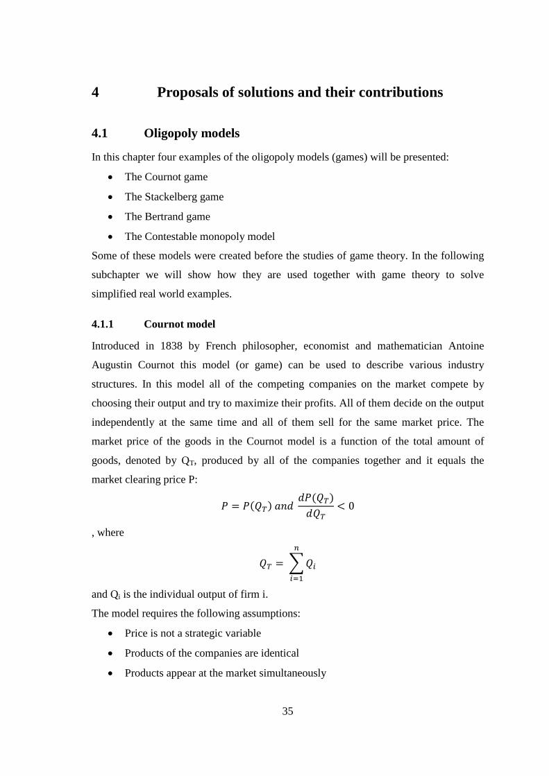
4 Proposals of solutions and their contributions
4.1 Oligopoly models
In this chapter four examples of the oligopoly models (games) will be presented:
• The Cournot game
• The Stackelberg game
• The Bertrand game
• The Contestable monopoly model
Some of these models were created before the studies of game theory. In the following
subchapter we will show how they are used together with game theory to solve
simplified real world examples.
4.1.1 Cournot model
Introduced in 1838 by French philosopher, economist and mathematician Antoine
Augustin Cournot this model (or game) can be used to describe various industry
structures. In this model all of the competing companies on the market compete by
choosing their output and try to maximize their profits. All of them decide on the output
independently at the same time and all of them sell for the same market price. The
market price of the goods in the Cournot model is a function of the total amount of
goods, denoted by QT, produced by all of the companies together and it equals the
market clearing price P:
𝑃 = 𝑃(𝑄𝑇) 𝑎𝑛𝑑 𝑑𝑃(𝑄𝑇)𝑑𝑄𝑇
< 0
, where
𝑄𝑇 = �𝑄𝑖
𝑛
𝑖=1
and Qi is the individual output of firm i.
The model requires the following assumptions:
• Price is not a strategic variable
• Products of the companies are identical
• Products appear at the market simultaneously
Page 36
36
• Firms do not cooperate
• The number of firms is fixed
• The market price decreases when the total output rises
(FUDENBERG and TIROLE, 1998)
The following example illustrates the use of this model.
Two firms form a duopoly on the gold mining market: We Mine and Shiny Gold. Both
of them sell the gold that they mine each month at a gold market. The quantity of gold
mined by We Mine will be denoted QWM and Shiny Gold’s quantity QSG. The market
price at the gold market is given by the following demand equation in €/ounce of 24-
karat gold:
𝑃 = �840 − 4 ∗ 𝑄𝑇 𝑖𝑓 0 ≤ 𝑄𝑇 ≤ 2100 𝑖𝑓 𝑄𝑇 > 210
Figure 4.1 Demand curve for the gold market
Each month both firms have to decide how much gold they want to mine – they have to
select a strategy. They decide at the same time and independently. The quantities are
given in thousands of ounces and revenue, cost and profit in thousands of euro.
Page 37
37
The mining and transporting costs of the companies are identical and are 600€/ounce.
Total costs for each company are:
𝑇𝐶𝑖 = 600 ∗ 𝑄𝑖 𝑓𝑜𝑟 𝑖 = 𝑊𝑒 𝑀𝑖𝑛𝑒, 𝑆ℎ𝑖𝑛𝑦 𝐺𝑜𝑙𝑑
Now, we can write the profit function for each of the gold mining companies.
Profit function for the We Mine company:
𝜋𝑖(𝑄𝑊𝑀) = �840 − 4 ∗ (𝑄𝑊𝑀 + 𝑄𝑆𝐺)� ∗ 𝑄𝑊𝑀 − 𝑄𝑊𝑀 ∗ 600
Profit function for the Shiny Gold company:
𝜋𝑖(𝑄𝑆𝐺) = �840 − 4 ∗ (𝑄𝑊𝑀 + 𝑄𝑆𝐺)� ∗ 𝑄𝑆𝐺 − 𝑄𝑆𝐺 ∗ 600
The profits are considered the payoffs in this game. The companies play a static game
with complete information (the profit functions are common knowledge).
4.1.1.1 Monopoly
To compare solutions to this game we will first assume that there is only one company -
We Mine. In this case its profit function will look like this:
𝜋𝑊𝑀(𝑄𝑊𝑀) = (840 − 4 ∗ 𝑄𝑊𝑀) ∗ 𝑄𝑊𝑀 − 𝑄𝑊𝑀 ∗ 600
After simplification:
𝜋𝑊𝑀(𝑄𝑊𝑀) = 240 ∗ 𝑄𝑊𝑀 − 6 ∗ 𝑄𝑊𝑀2
To find the optimal output, we now only have to find the maximum of the profit
function using simple calculus. To find the maximum we have to put the derivative of
the profit function equal to 0:
240 − 12 ∗ 𝑄𝑊𝑀 = 0
And the output associated with the maximum profit is:
𝑄𝑊𝑀 = 20
Profit at this output level is equal to:
𝜋𝑊𝑀(20) = 240 ∗ 20 − 6 ∗ 202 = 2400
So in the case of one company on the market, this company would produce 20 000
ounces of gold each month and make a profit of 2 400 000€.
Page 38
38
Figure 4.2 Graph of the profit function for firm We Mine
4.1.1.2 Duopoly
We can return to the problem with two competing companies. To illustrate the problem
in a better fashion, we can use the isoprofit curves. Isoprofit curves show all of the
different levels of outputs of both mining companies where one of them makes a certain
level of profit. For a given profit of πx for the company We Mine, the isoprofit curve for
the Shiny Gold company is the following function:
𝑄𝑆𝐺 = 60 −𝜋𝑥
4 ∗ 𝑄𝑊𝑀− 𝑄𝑊𝑀
The following graph illustrates the isoprofit curves for the company We Mine for these
levels of profit 0, 250, 500, 1000 and 2000.
Page 39
39
Figure 4.3 Isoprofit curves for We Mine
Now we have to find the best responses for the level of output selected by the
competitor. For example if Shiny Gold selects the output of 0 units, then the best
response for the We Mine company will be to select the output of 20 as if it was alone
on the market (actually they select their output at the same time, so the best response
output will be selected next month). For each non-zero output level we have to find an
isoprofit curve that is tangent to the horizontal line of the output at the height of QSG.
For example if the Shiny Gold’s output is 30, then the best response for the We Mine
will be to select the output of 15. It is illustrated in Figure 4.4.
Page 40
40
Figure 4.4 Best response for the Shiny Gold’s output of 30
To find the best response for each one of the levels of output we have to find the best
response functions for both companies, that is, the functions that assign a level of
output to each level of competitor’s output in a way to maximize profit. We can
calculate this function for the We Mine by taking the partial derivative of their profit
function with respect to QWM and calculating the level of output when it equals 0.
𝜕𝜋𝑊𝑀(𝑄𝑊𝑀,𝑄𝑆𝐺)𝜕𝑄𝑊𝑀
= 240 − 8 ∗ 𝑄𝑊𝑀 − 4 ∗ 𝑄𝑆𝐺 = 0
Solving for QWM, the best response function for We Mine is:
(4.1) 𝑄𝑊𝑀𝐵𝑅 (𝑄𝑊𝑀,𝑄𝑆𝐺) = 30 − 0.5 ∗ 𝑄𝑆𝐺
Shiny Gold’s best response function:
(4.2) 𝑄𝑆𝐺𝐵𝑅(𝑄𝑊𝑀,𝑄𝑆𝐺) = 30 − 0.5 ∗ 𝑄𝑊𝑀
To find the quantities that the companies will choose according to Cournot model, we
now just have to find the intersection of these two best response functions. We can
depict it graphically as shown in Figure 4.5.
Page 41
41
Figure 4.5 Intersection of the best response functions
We can also find the equilibrium mathematically by solving a system of linear equations
4.1 and 4.2. The solution is that both the firms will mine 20 units (20 000ounces), sell
them for a price of 680€/ounce and earn a profit of 1600 (1 600 000€). This is the
Cournot duopoly equilibrium for this game. This is also the Nash equilibrium of this
game as both players maximize their profits when they are playing their best responses
and they are both playing their best responses in this point. We can also receive the
same result by iteratively eliminating dominated strategies.
But Cournot model can be used to model more than monopoly and duopoly market a
structure. By increasing the number of companies and decreasing their market share we
are also able to model perfect competition.
4.1.1.3 Perfect competition
We can modify the previous gold mining example by adding more firms to the market.
Now for N gold mining companies the profit function for the i-th company will be given
by.
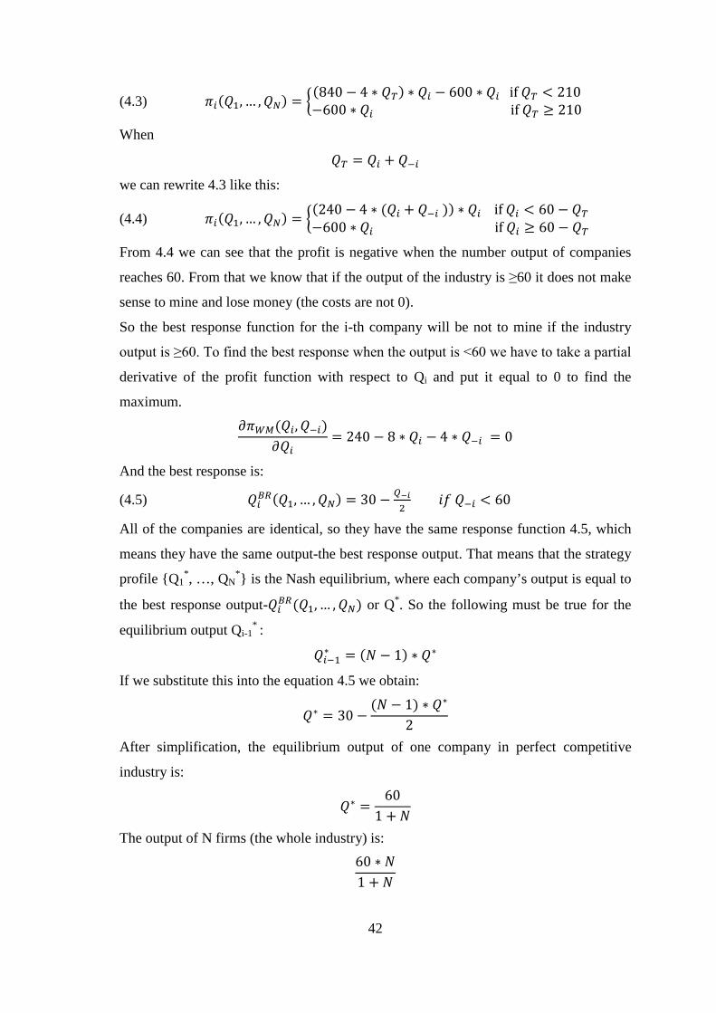
Page 42
42
(4.3) 𝜋𝑖(𝑄1, … ,𝑄𝑁) = �(840 − 4 ∗ 𝑄𝑇) ∗ 𝑄𝑖 − 600 ∗ 𝑄𝑖 if 𝑄𝑇 < 210−600 ∗ 𝑄𝑖 if 𝑄𝑇 ≥ 210
When
𝑄𝑇 = 𝑄𝑖 + 𝑄−𝑖
we can rewrite 4.3 like this:
(4.4) 𝜋𝑖(𝑄1, … ,𝑄𝑁) = �(240 − 4 ∗ (𝑄𝑖 + 𝑄−𝑖 )) ∗ 𝑄𝑖 if 𝑄𝑖 < 60 − 𝑄𝑇−600 ∗ 𝑄𝑖 if 𝑄𝑖 ≥ 60 − 𝑄𝑇
From 4.4 we can see that the profit is negative when the number output of companies
reaches 60. From that we know that if the output of the industry is ≥60 it does not make
sense to mine and lose money (the costs are not 0).
So the best response function for the i-th company will be not to mine if the industry
output is ≥60. To find the best response when the output is <60 we have to take a partial
derivative of the profit function with respect to Qi and put it equal to 0 to find the
maximum.
𝜕𝜋𝑊𝑀(𝑄𝑖,𝑄−𝑖)𝜕𝑄𝑖
= 240 − 8 ∗ 𝑄𝑖 − 4 ∗ 𝑄−𝑖 = 0
And the best response is:
(4.5) 𝑄𝑖𝐵𝑅(𝑄1, … ,𝑄𝑁) = 30 − 𝑄−𝑖2
𝑖𝑓 𝑄−𝑖 < 60
All of the companies are identical, so they have the same response function 4.5, which
means they have the same output-the best response output. That means that the strategy
profile {Q1*, …, QN
*} is the Nash equilibrium, where each company’s output is equal to
the best response output-𝑄𝑖𝐵𝑅(𝑄1, … ,𝑄𝑁) or Q*. So the following must be true for the
equilibrium output Qi-1* :
𝑄𝑖−1∗ = (𝑁 − 1) ∗ 𝑄∗
If we substitute this into the equation 4.5 we obtain:
𝑄∗ = 30 −(𝑁 − 1) ∗ 𝑄∗
2
After simplification, the equilibrium output of one company in perfect competitive
industry is:
𝑄∗ =60
1 + 𝑁
The output of N firms (the whole industry) is: 60 ∗ 𝑁1 + 𝑁
Page 43
43
For N->∞ the output of the industry equals 60 000 ounces of gold with a profit of 0.
The problem of this model is that in real world the companies usually do not compete
by setting the quantities that they produce and they set their own prices.
4.1.2 Stackelberg model
This model (or game) was introduced by Heinrich Freiherr von Stackelberg, a German
economist, in 1934. It models a duopoly in which there is a company that is a leader and
another one that is a follower. The game is sequential; the leader moves first and sets
the quantity he is going to produce. Then the follower observes this and sets his
quantity. Other important assumptions are:
• Both players are perfectly informed about the game structure and payoffs
• The leader knows that the follower will follow him
We will demonstrate the usage of this model on the following example:
There is a monopolist, Metalheads T’s (MT), producing T-shirts for a certain niche
market. Each month he has to decide how many T-shirts he wants to order from the
manufacturer in China. A new company, Brutal T-shirts (BT), wants to enter this
market. They can observe how many T-shirts the incumbent company is going to
produce and after that they have to decide how many T-shirts they will produce. The
monopolist knows that this competitor will make its decision based on their decision
and they have to set their quantity while keeping that in mind. For the sake of simplicity
the cost structure is the same for both companies. The costs associated with making one
T-shirt are 1€. The demand for these T-shirts for the specific market is given by this
demand curve equation:
(4.6) 𝑃 = 801 − 2 ∗ 𝑄
Page 44
44
Figure 4.6 Demand curve for the T-shirts market
4.1.2.1 Monopoly
The following solution is for the case that the monopolist is alone on this market. How
many T-shirts will he produce? He will produce the amount of T-shirts that gives him
the highest profit. His profit function is:
𝜋(𝑃,𝑄) = (𝑃 − 1) ∗ 𝑄
After substituting in the demand curve equation 4.6:
𝜋(𝑄) = (801 − 2 ∗ 𝑄 − 1) ∗ 𝑄
After simplification:
𝜋(𝑄) = 800 ∗ 𝑄 − 2 ∗ 𝑄2
To find the maximum we have to take the derivative with respect to Q and put it equal
to 0:
𝜕𝜋(𝑄)𝜕𝑄
= 800 − 4 ∗ 𝑄 = 0
Page 45
45
𝑄∗ = 200
The optimum production for the monopolist is 200 T-shirts, which earns him a profit of:
𝜋(200) = 800 ∗ 200 − 2 ∗ 2002 = 80 000€
So if the monopolist was on the market alone, he would produce 200 T-shirts, sell each
for the price of 400€ and make a profit of 80 000€.
4.1.2.2 Duopoly
Now, the monopolist has to consider that after he makes his decision, he is going to be
followed by the competitor. The resulting game is a sequential (dynamic) game in
which the leader moves first and the follower moves second. The production of MT is
QMT and the BT is QBT, Q= QMT+ QBT. The demand equation now changes to:
𝑃 = 801 − 2 ∗ (𝑄𝑀𝑇 + 𝑄𝐵𝑇)
The profit equation of the monopolist now depends on both QMT and QBT. The profit
equation looks like this:
𝜋𝑀𝑇 = (801 − 2 ∗ (𝑄𝑀𝑇 + 𝑄𝐵𝑇) − 1) ∗ 𝑄𝑀𝑇
After simplification:
(4.7) 𝜋𝑀𝑇 = 800 ∗ 𝑄𝑀𝑇 − 2 ∗ 𝑄𝑀𝑇2 − 2 ∗ 𝑄𝑀𝑇 ∗ 𝑄𝐵𝑇
The profit equation of BT is:
𝜋𝐵𝑇 = 800 ∗ 𝑄𝐵𝑇 − 2 ∗ 𝑄𝐵𝑇2 − 2 ∗ 𝑄𝑀𝑇 ∗ 𝑄𝐵𝑇
To solve this game we have to reason backwards. First we have to find out how will BT
react to MT’s output choice. To find the output which maximizes profit of BT we have
to take the partial derivative of their profit function with respect to QBT and put it equal
to 0. The QMT is considered a constant at this point – the monopolist has already set the
quantity.
𝜕𝜋𝐵𝑇(𝑄𝑀𝑇 ,𝑄𝐵𝑇)
𝜕𝑄𝐵𝑇= 800 − 4 ∗ 𝑄𝐵𝑇 − 2 ∗ 𝑄𝑀𝑇 = 0
(4.8) 𝑄𝐵𝑇𝐵𝑅 = 200 − 𝑄𝑀𝑇2
The equation 4.8 gives us the answer to the question: How many T-shirts is BT going to
make given that MT makes QMT T-shirts? It is their best response function. We assume
the perfect knowledge of the game, so the leader - MT knows this function. His profit
Page 46
46
depends on the choice of BT’s output so we can substitute the BT’s response function
into MT’s profit function 4.7.
𝜋𝑀𝑇 = 800 ∗ 𝑄𝑀𝑇 − 2 ∗ 𝑄𝑀𝑇2 − 2 ∗ 𝑄𝑀𝑇 ∗ (200 −𝑄𝑀𝑇
2)
After simplification:
(4.9) 𝜋𝑀𝑇 = 400 ∗ 𝑄𝑀𝑇 − 𝑄𝑀𝑇2
To find the level of output which gives MT the maximum profit, we just have to find
the maximum of the 4.9 function.
𝜕𝜋𝑀𝑇(𝑄𝑀𝑇)𝜕𝑄𝑀𝑇
= 400 − 2 ∗ 𝑄𝑀𝑇 = 0
𝑄𝑀𝑇 = 200
MT produces 2000 T-shirts and makes a profit of:
𝜋𝑀𝑇 = 400 ∗ 200 − 2002 = 40 000€
The price for one T-shirt in this situation is 200€.
When we compare the profit of the monopolist when he is alone and when he has a
competitor, we see that his profit was reduced to half.
BT will make:
𝑄𝐵𝑇 = 200 −200
2= 100
T-shirts and make a profit equal to half of MT’s profit (half of the number of T-shirts
times the same price), which is 20 000€. None of the players can do any better by
changing their output -> it is a Nash equilibrium.
This model shows that the entry of a new competitor reduces prices and also profits for
the incumbent firm.
This model also has another important aspect - the company that moves first always
makes twice the money of the company that moves last. The first company has the first
mover advantage. This is not generally true for every game, but it is a property of a
portion of them.
4.1.3 Bertrand model
This model (or game) was introduced by Joseph Louis François Bertrand, a French
mathematician. The difference between Bertrand and Stackelberg or Cournot model is
Page 47
47
that the companies in Bertrand model compete with prices instead of quantities. The
Bertrand game is a static game with perfect information. The companies make their
decisions independently and simultaneously. Other assumptions:
• Product is homogeneous.
• Customers are rational – they buy for the lowest price
To illustrate the usage of this model, consider the following example:
There are two chemical factories in city that form a duopoly on the market with sulfuric
acid - Acidity (A) and Bang (B). We assume that both of them produce sulfuric acid
with constant marginal costs of 5€ per liter of acid and do not have any fixed costs.
Companies make their prices known independently and at the same time. The product is
exactly the same from both companies, so the customer only cares about the pricing. If
the prices are the same, the companies split the market. There is a positive demand for
the sulfuric acid at a price of 5€ per liter.
There is no point in selling under the marginal costs of producing the acid so we do not
have to consider prices below the 5€/lt level. If company A sets its prices at for example
6€/lt than it is reasonable for the management of B to set the price slightly lower than
6€/lt, capture the whole market and make profit. If they choose a price higher than A,
then they will have zero market share and make zero profit. If they choose the same
price as A, then they will only capture half of the market and make lower profit then
they would have made if they had chosen a lower price than A. But management of A
has to consider the same. This concludes that both companies will charge the price of
6€/lt, which is equal to their marginal costs and is the Nash equilibrium as neither of the
companies can do any better.
To allow the companies to make profit in the Bertrand model we have to change our
assumptions about the game. One of the possible modifications is to limit the capacities
of the competitors.
4.1.4 Contestable markets
This is the newest of the presented models (or games) introduced by William Jack
Baumol, American economist, in 1982. A contestable market is a market where only a
Page 48
48
small number of firms operate, but they cannot make excessive profits as they are under
the threat of entry by potential competitors.
“A contestable market is one for which:
1. An unlimited number of potential firms exist that can produce the
(homogeneous) with a common technology.
2. Entry in to the market does not involve a sunk cost, that is, an expenditure that
cannot be completely recovered should the firm decide to leave the market.
3. Firms are price-setting Bertrand competitors.
A contestable monopoly is a contestable market with a Nash equilibrium in which
exactly one firm supplies the entire market. In a contestable monopoly, since the
threat of entry drive monopoly rents to zero, the firm will produce the greatest
output at which it remains financially viable. This is referred to as a second-best
output.”
(BIERMAN and FERNANDEZ, 1998, p.52-53)
An example for this kind of market can be a market with taxi services in a small town.
Consider two taxi companies: AB Taxi (AB) and Okey Taxi (OK). To provide the
service, the companies only need to have a number of cars and drivers (we will assume
that there is no need for a special license). There are fixed costs associated with buying
or leasing the cars needed, but they are not sunk costs as the cars can be sold or used in
another city. QAB, PAB, QOK and POK are the respective quantities of transported
passengers and prices for one ride for both companies. The number of clients is in
hundreds per month and prices are in € per ride. The companies have the same costs,
which are:
𝐶 = �4 + 4 ∗ 𝑄 𝑖𝑓 𝑄 > 00 𝑖𝑓 𝑄 = 0
If one of the companies decides to quit the market, they can sell their cars and that way
avoid any losses (no sunk costs). Both companies announce their prices at the same
time. The demand curve is given by the equation:
𝑃 = 15 − 2.5 ∗ 𝑄
Page 49
49
Figure 4.7 Demand and average costs curves for the contestable monopoly
From the picture we can see that at the price of 5€ per ride there is a demand of a 400
customers. Now, we will show that there are two Nash equilibrium strategies in this
game for both companies (the companies are the same and so the strategies are
symmetrical):
• AB sets its price to 5€ and transports 400 passengers and OK transports no one.
• OK sets its price to 5€ and transports 400 passengers and AB transports no one.
It is enough to show that the first strategy is a Nash equilibrium and that neither of the
players can do any better than playing that strategy. If OK sets its prices lower than 5€
they will catch the whole market but they will lose money on it, unless they refuse to
transport anyone, as the average costs are equal to 5€. If OK sets its prices to 5€ exactly,
they will transport half of the passengers and also lose money, unless they refuse to
transport anyone. If they set their prices higher than 5€, they will not transport anyone
as all the passengers will go to the competition. They will not make any profit, but if
they sell its cars to another company (or use them in a different city) they will also not
lose any money. So it is the optimal strategy for OK to not transport anyone and sell its
cars. It is also optimal for AB to set its prices to 5€, as the lower price would make them
Page 50
50
lose money on transporting and higher price would make room for a competitor to enter
the market and make positive profits.
The important property of this model is that the possibility of entry (not the actual
entry) is in some special markets enough to keep the prices low enough to discourage
potential competitors from entering the market.
4.1.5 Summary of the oligopoly models
Both Stackelberg and Cournot models model companies competing by setting the
quantities they want to produce, while Bertrand model models them competing on price.
Each model has its uses depending on the structure of the market whose behavior we try
to predict. All of these models in the form given here are too simple to model real life
markets. The important assumptions to consider are the one-time nature of the price
setting and also the homogeneity of the companies’ products in these games which is in
most cases not true in real markets.
4.2 Economic views comparison
In this chapter different ways of reasoning will presented on an example of a strategic
investment.
There are two companies on a pharmaceutical market – Friendly Pharm (FP) and
Medicinal Goodness (MG). Both of them produce an analgesic medicine. These two
products are perfect substitutes. Quantities are in kilograms, revenues, costs and profit
are in thousands of euro and prices are in €/kg. These companies both have the same
marginal costs, MC1=MC2=MC equal to:
𝑀𝐶 = 25
It means that it costs them 25€ to produce one kilogram. The demand curve for these
products is:
(4.10) 𝑃 = 109 − 16∗ 𝑄
Q is the sum of quantities that the companies produce:
𝑄 = 𝑄𝐹𝑃 + 𝑄𝑀𝐺
They produce the same quantity of these products, QFP=QMG=168, which is the Cournot
equilibrium output. At this output the price of one kilogram is:
Page 51
51
𝑃 = 109 − 56 = 53€
They both make a yearly profit of:
𝜋 = (53 − 25) ∗ 168 = 4704
It means that the profit of each company equals 4 704 000€.
FP is considering an investment in a new manufacturing process in their factory. This
investment would lower their marginal costs to:
𝑀𝐶𝐹𝑃 = 20
The cost of this new process is 1 000 000€.
Now we will compare three different perspectives on this investment:
• “Accountant’s” perspective
• “Economist’s” perspective
• “Game theorist’s” perspective
4.2.1 Accountant’s point of view
From this perspective we will count the money that this process will save us and
compare it with the cost of the machine.
We produce 168 kilograms with costs 5€ lower than before, so we save:
168 ∗ 5 = 840
The savings are 840 000€ in variable costs, but the cost of the new process is
1 000 000€. We can see that the costs of the new process are much higher than the
savings it brings. So, in conclusion, we advise not to invest in this process as it will
bring no advantage.
4.2.2 Economist’s point of view
From this perspective we can see that when production costs are lowered by the new
process, we not only save money, but we can also produce more. Our residual demand
curve is:
(4.11) 𝑃𝑅 = 109 − 16∗ (𝑄𝐹𝑃 + 168) = 81 − 1
6∗ 𝑄𝐹𝑃
Quantity which maximizes profit is in the point where marginal revenue equals
marginal costs:
(4.12) 𝑀𝑅𝐹𝑃 = 𝑀𝐶𝐹𝑃
Page 52
52
We already know the marginal costs. We can calculate total revenue, denoted by TR, by
multiplying 4.11 with the produced quantity QFP:
(4.13) 𝑇𝑅𝐹𝑃 = 𝑃𝑅 ∗ 𝑄𝐹𝑃 = �81 − 16∗ 𝑄𝐹𝑃� ∗ 𝑄𝐹𝑃 = 81 ∗ 𝑄𝐹𝑃 −
16∗ 𝑄𝐹𝑃2
From 4.13 we can calculate the marginal revenue by taking its derivative:
𝑀𝑅𝐹𝑃 =𝜕𝑇𝑅𝐹𝑃(𝑄𝐹𝑃)
𝜕𝑄𝐹𝑃= 81 −
13∗ 𝑄𝐹𝑃
Now we substitute it into 4.12:
81 −13∗ 𝑄1 = 20
And we obtain QFP:
𝑄𝐹𝑃 = 183
We can also solve it graphically:
Figure 4.8 Graphical solution – „economist‘s“
With the output of 183 kilograms the new price is:
𝑃 = 109 −16
(183 + 168) = 50.5€
And the profit is:
𝜋𝐹𝑃 = (50.5 − 20) ∗ 183 = 5581.5
Page 53
53
The new profit is 5 581 500€. The difference between the profit before adopting the
process and after adopting is 877 500€ which is still lower than the costs of the new
process. So, in conclusion, we again advise not to invest in this process as it will bring
no advantage.
4.2.3 Game theorist’s point of view
The previous view did not take into consideration the opponent’s reaction to our
increased production. We will model the situation as a sequential game. First the FP
decides whether to invest or not, then they play Cournot game. To solve this game we
can use backwards induction. To find the payoffs, we have to calculate the Cournot
Nash equilibrium of this game. To find it, we have to find the best response function for
both companies. The best response functions for this example are:
𝑄𝐹𝑃𝐵𝑅(𝑄𝐹𝑃,𝑄𝑀𝐺) =534 − 𝑄𝑀𝐺
2
𝑄𝑀𝐺𝐵𝑅 (𝑄𝐹𝑃,𝑄𝑀𝐺) =504 − 𝑄𝐹𝑃
2
When we solve this system of equations, we will get the following equilibrium
quantities:
𝑄𝐹𝑃 = 188
𝑄𝑀𝐺 = 158
We can also solve it graphically:
Page 54
54
Figure 4.9 Graphical solution – „game theorist‘s“
The price is now:
𝑃 = 109 −16∗ (188 + 158) = 51.333€
Now with the output of 188 kilograms the profit is:
𝜋𝐹𝑃 = (51.333 − 20) ∗ 188 = 5890.604
Now we see that the payoff from not investing in this new process is 4 704 000€ and the
payoff from investing is 5 890 604€ - 1 000 000€ = 4 890 604€. The optimal decision is
to invest in this new process. So, in conclusion, we advise to invest in this process as it
will bring increased profit.
4.3 Role of uncertainty in decision making
In this chapter the necessary tools needed to treat games involving uncertainty will be
recalled. First a concept of mixed strategies, strategies where each move is assigned a
Page 55
55
probability, will be introduced. Later we will describe games with imperfect and
incomplete information and tools needed to solve them.
4.3.1 Mixed strategies
Each strategy has to assign an action for each decision – which path to take. But this
does not have to be defined absolutely. The action to be taken can be defined using
probabilities – each action will be played with a certain probability. Let us explain the
issue on the following game.
Two players named Alice (A) and Bob (B) are playing a game of rock-paper-scissors.
The loser has to pay one euro to the winner. Bob brags to Alice that he is such a good
player of this game, that if they tie with a rock, it will count as a win for her, and he will
pay her one euro. The payoffs for this game are:
Rock (q1) Paper (q2) Scissors (q3)Rock (p1) (1, -1) (-1, 1) (1, -1)Paper (p2) (1, -1) (0, 0) (-1, 1)Scissors (p3) (-1, 1) (1, -1) (0, 0)Expected payoff to Bob -p1-p2+p3 p1-p3 -p1+p2
Alice
Bob
Table 4.1 Payoffs for the modified rock-paper-scissors
4.3.1.1 Solution with pure strategies
The pure strategies for this game are:
• Always play rock – Rock strategy
• Always play paper – Paper strategy
• Always play scissors – Scissors strategy
We can try finding pure strategy equilibrium for this game:
• If A plays Rock strategy, the best response from B is to play Paper. Given that B
plays Paper, the best response from A is to play Scissors. {Rock, Paper} is not
an equilibrium strategy profile.
• If A plays Paper strategy, the best response from B is to play Scissors. Given
that B plays Scissors, the best response from A is to play Rock. {Paper,
Scissors} is also not an equilibrium strategy profile.
Page 56
56
This way we can check all of the possible strategy profiles and we will find out that
there is no equilibrium for this game using only pure strategies.
4.3.1.2 Solution with mixed strategies
Now the players will choose each action with a certain probability – they will play
mixed strategies. If the mixed strategies contain all of the player’s pure strategies, they
are completely mixed strategies. To find the optimal probabilities with which the
player should play each action we have to calculate the expected payoffs first. Expected
payoff of a strategy is the sum of the probability of each action multiplied by its payoff.
The probabilities for player A playing rock, paper or scissors will be denoted p1, p2 and
p3 respectively and for player B q1, q2 and q3 respectively. It is important that
p1+p2+p3=1, and q1+q2+q3=1. The equations for the expected payoffs are in the
following table:
Rock (q1) Paper (q2) Scissors (q3) Expected payoff to AliceRock (p1) (1, -1) (-1, 1) (1, -1) q1-q2+q3
Paper (p2) (1, -1) (0, 0) (-1, 1) q1-q3
Scissors (p3) (-1, 1) (1, -1) (0, 0) q1-q2+q3
Expected payoff to Bob -p1-p2+p3 p1-p3 -p1+p2
Alice
Bob
Payoffs: (Alice, Bob)
Table 4.2 Expected payoffs for the modified rock-paper-scissors
After solving the system of equations we will get the following solution:
p1=1/3, p2=4/9, p3=2/9, q1=1/3, q2=2/9, q3=4/9. It means that player A will play rock
with probability of 1/3, paper with probability of 4/9 and scissors with probability of 2/9
and respectively for player B.
This is the Nash equilibrium with mixed strategies. It means that if both players play the
actions with those probabilities, they are both equally likely to win.
An important fact about games and mixed strategies is given by:
“Every game with a finite number of players, each of whom has a finite number of pure
strategies, possesses at least one Nash equilibrium, possibly in mixed strategies.”
(BIERMAN and FERNANDEZ, 1998, p.220)
Page 57
57
4.3.2 Games with imperfect information
To describe the games with imperfect information we employ the following example:
We have a monopolist market for smart phones. There is an incumbent firm - Pear
Mobile (PM) and a firm that wants to enter this market - Small Mobile (SM). Both
companies have perfect information about the game structure and payoffs. The game
consists of two stages. In first stage the entrant decides whether to enter the market or
not. If the entrant enters the market the game goes into second stage. In the second stage
PM decides whether to fight the entrant and invest in a huge TV advertisement
campaign or not fight. There are costs associated with entering the market. It is a
dynamic game with perfect information. Payoffs are in millions of euro. The game tree
is depicted in Figure 6.1.
Figure 4.10 Game tree for the entry deterrence game with perfect information
4.3.2.1 Solution with perfect information
We can find the solution for this game using the backwards induction. Given that SM
will choose to enter, the best response for PM is to not fight them and get a payoff of
70. As both players have complete knowledge of the game, SM observes this and
chooses to enter the market and gets payoff of 20. So the strategy profile {enter, do not
fight} is the subgame perfect equilibrium for this game. If the incumbent firm says that
Page 58
58
they are going to fight if the entrant enters, they are making an incredible threat, as it
is not in their best interest to actually fight SM when they enter.
4.3.2.2 Solution with imperfect information
Now we will modify this example by stating that if SM enters and PM fights, there is a
20% chance that the ad campaign will be a great success. That means it will lure more
customers and PM will make more money when fighting than when not fighting. It will
be modeled by introducing the player Nature into the game which decides the outcome
of the campaign if SM enters and PM decides to fight. Neither player knows the
outcome of the campaign. This is a game with imperfect information. The game tree
now looks like this (terminal nodes are labeled to make the next step clearer):
Figure 4.11 Game tree for the entry deterrence game with incomplete information
To solve this game with probabilities we need to modify the backwards induction
algorithm to work with Nature’s moves.
4.3.2.3 Modified backwards induction
We need to modify the first three steps of the backwards induction algorithm like this:
„
1. Start at the terminal nodes of the game and trace each one to its immediate
predecessor, which will be a decision node for some player. These decision
nodes are either “trivial”, “basic”, or “complex”. A decision node is basic if
each of its branches you can either reach exactly one terminal node or a basic
Page 59
59
decision node belonging to Nature. A basic node with only one branch is trivial.
A decision node is complex if, starting from one of its branches, you can reach
one or more decision nodes of strategic players or a complex deicison node
belonging to Nature. If you reach a trivial decision node, then keep moving up
the tree until you reach either a complex or nontrivial basic decision node or
until you can go no further.
2.
a. If the basic node belongs to Nature, then when this node is reached, the
outcome is determined at random using predetermined probabilities.
Calculate the expected payoff for each player using these probabilities.
b. If the basic node belongs to a strategic player, then find the optimal
move by comparing the payoffs the player obtains at each terminal node
reached from this decision node. Note that every path between a basic
decision node A and a terminal node B starts at a unique branch of A.
The branch that leads to the highest payoff for the player is the optimal
move to make at that node.
3.
a. Erase all the branches of the basic decision nodes belonging to Nature
that you examined in step 2a. Each of these decision nodes now becomes
a terminal node. Assign to these terminal nodes the expected payoffs you
calculated in step 2a.
b. Erase all the non-optimal branches that originate from each of the basic
decision nodes you examined in step 2b. Each of these basic decision
nodes becomes trivial. “
(BIERMAN and FERNANDEZ, 1998, p.212-213)
Now we apply this modified backwards induction algorithm to the entry deterrence
game with incomplete information. When we come to the Nature’s move, we calculate
the expected payoff from terminal nodes T4 and T3. The expected payoff for PM is 0.8 *
60 + 0.2 * 120 = 48 + 24= 72 and for SM it is 0.2 * (-10) + 0.8 * (-10) = -10. After
removing the branches belonging to Nature, the tree now looks like this:
Page 60
60
Figure 4.12 Pruned game tree for the entry deterrence game with incomplete information
Now we can see that PM’s best move is to fight with a payoff of 72 compared to 70
when not fighting. After eliminating the corresponding branch, the tree now looks like
this:
Figure 4.13 Game tree for the entry deterrence game with incomplete information after more pruning
From this game tree we can see that SM’s optimal move is not to enter the market and
get a payoff of 0, compared to -10 when entering. We have found the subgame perfect
equilibrium and it is {fight, do not enter}.
4.3.3 Games with incomplete information
In this subchapter we will analyze and solve static and dynamic games with incomplete
information.
Page 61
61
4.3.3.1 Static games with incomplete information – static Bayesian games
Static game with incomplete information is called a Bayesian game. The normal form of
the Bayesian game differs from the normal form of a game with complete information.
It also involves player types and prior beliefs. The player type is information which
each player knows about him, but not about other players and it determines his payoff
function. In the case of previous example we can say that player PM can be of two
types, one with successful campaign and the other one with a not successful campaign.
Player’s prior beliefs about other players’ types represent the probabilities for each
possible type of other players.
(GIBBONS, 1992)
We will modify the previous entry deterrence game again. This time PM has done
extensive market research and knows for sure, what impact the campaign is going to
have. One possible outcome is that the campaign will be a great success and PM will
earn high profit. Another is that the campaign will be a failure and will let the
competitor enter the market and make a profit. In this game PM moves simultaneously
with SM and decides whether to invest in the campaign or not. At the same time SM
independently decides whether to enter the market or not. SM did their research too, but
they only know that with 60% probability the campaign will be a great success and with
40% probability a failure. It is a static game with incomplete information, also called a
static Bayesian game. SM does not know if they are playing a game where the PM’s
campaign will be a great success or a game where PM’s campaign will be a failure. PM
knows this. The payoffs of these different games are given in Table 6.3.
Enter Don't enter Enter Don't enterDo campaign (100, -10) (120, 0) (60, -10) (80, 0)Don't do campaign (70, 20) (90, 0) (70, 20) (90, 0)
Payoffs: (PM, SM)
SM
PM
Great success FailureSM
Table 4.3 Payoffs for the static game with incomplete information
Page 62
62
We can identify that in both of these games PM has a dominant strategy. In the game,
where the campaign is a great success PM’s dominant strategy is to Do campaign. In the
game where the campaign is a failure Don’t do campaign is PM’s dominant strategy.
SM does not have a dominant strategy. To solve this game we have to use the Harsanyi
transformation.
Harsanyi transformation
The Harsanyi transformation, formulated by John Harsanyi in 1967 transforms a
game with incomplete information into a game with complete but imperfect
information. This transformation is done in this way: first the Nature decides the types
of each player based on the probability of each type. Then Nature reveals to each player
his own type. After that both players make their decisions simultaneously and receive
their payoffs based on their types.
(GIBBONS, 1992)
To find the optimal solution for the game after the Harsanyi transformation we have to
find the Bayesian Nash equilibrium.
Bayesian Nash equilibrium
In Bayesian games players try to maximize their conditional expected utilities. The
conditional expected utilities are calculated for every strategy profile from the expected
utilities which depend on types of players, multiplied by conditional probability
calculated from prior beliefs about the players’ types.
(BIERMAN and FERNANDEZ, 1998)
How to do the calculations is beyond the scope of this work. See the above mentioned
literature for example.
“Concepts of dominant strategy (both strict and weak), dominant strategy equilibrium,
iterated dominant strategy equilibrium, and Nash equilibrium all extend naturally to this
new class of games if we replace the word “payoff” with “conditional expected
utility”.”
(BIERMAN and FERNANDEZ, 1998, p.278)
The extension of Nash equilibrium to Bayesian games is called the Bayesian Nash
equilibrium.
Page 63
63
The entry deterrence game can now be represented by the following table using the
conditional expected utilities:
Enter Don't enter(Do campaign, Do campaign) ((100, 60), (-10)) ((120, 80), (0))(Do campaign, Don't do campaign) ((100, 70), (2)) ((120, 90), (0))(Don't do campaign, Do campaign ) ((70, 60), (8)) ((90, 80), (0))(Don't do campaign, Don't do campaign) ((70, 70), (20)) ((90, 90), (0))
SM
Conditional Expected Utilities: ((successful PM, not successful), (SM))
PM
Table 4.4 Conditional expected utilities for the static game with incomplete information
Now we can find the strategy profile that is the Bayesian Nash equilibrium. If we
evaluate all of the strategy profiles we can find that the strategy profile {(Do campaign,
Don't do campaign), (Enter)} is the only Bayesian Nash equilibrium for this game.
4.3.3.2 Dynamic games with incomplete information
Again the entry deterrence game will be slightly modified. This time PM knows
whether the campaign will be a great success or a failure and has to make the decision
to do it or not. But the campaign is also more expensive. PM is of two types: Successful
and Unsuccessful. SM has done some market research and has prior beliefs that with the
probability of 25% the campaign will be a great success and with the probability of 75%
it will be a failure. Players move in sequence, first PM has to decide whether to do the
campaign or not. After that SM, observing PM’s decision but not knowing their type,
has to make a decision whether to enter the market or not. It is a dynamic game with
incomplete information. We will use the Harsanyi transformation and model this game
as a game with imperfect information where Nature moves first and decides the type of
PM. The game tree with payoffs is depicted in Figure 6.5.
Page 64
64
Figure 4.14 Game tree for the dynamic game with incomplete information
The dashed rectangles around SM’s decision nodes represent two different information
sets. At the time SM is making their decision to enter the market or not, they do not
know the type of PM, they only know their previous decision to do the campaign or not.
PM has two decision two make: whether to do the campaign when they know it will be
successful and whether to do the campaign when they know it will be a failure. SM has
two decisions to make: whether to enter the market when PM does the campaign and
whether to enter the market when PM does not do the campaign. Now we have to
calculate the conditional expected payoffs and find the Nash equilibria of this game.
The normal form representation of the game:
Page 65
65
(Enter, Enter)
(Enter, Don't Enter)
(Do campaign, Do campaign) ((70, 30), (-10)) ((70, 50), (-2.5))(Do campaign, Don't do campaign) ((70, 70), (12.5)) ((70, 90), (-2.5))(Don't do campaign, Do campaign ) ((70, 30), (-2.5)) ((70, 50), (5))(Don't do campaign, Don't do campaign) ((70, 70), (20)) ((70, 90), (5))
(Don't Enter, Enter)
(Don't Enter, Don't Enter)
(Do campaign, Do campaign) ((90, 30), (-7.5)) ((90, 50), (0))(Do campaign, Don't do campaign) ((90, 70), (15)) ((90, 90), (0))(Don't do campaign, Do campaign ) ((90, 30), (-7.5)) ((90, 50), (0))(Don't do campaign, Don't do campaign) ((90, 70), (15)) ((90, 90), (0))
SM
PM
Conditional Expected Payoffs: ((successful PM, not successful), (SM)) Table 4.5 Normal form of the dynamic game with incomplete information
This game has two Nash equilibria: {(Don’t do campaign, Don’t do campaign), (Enter,
Enter))}, {(Do campaign, Don’t do campaign), (Don’t enter, Enter))}. To find the one
which does not involve incredible threats, we have to find the subgame perfect
equilibrium. But in this game, the whole game is one subgame, so both strategy profiles
are subgame perfect equilibria. We have to find the perfect Bayesian equilibrium.
Bayesian updating
Important notion is that SM does not know PM’s type, but has some belief about it. SM
assigns probabilities for each of the information sets (possible PM types) and this is
called the belief profile. There are two nontrivial information sets in the previous
example - Do campaign and Don’t do campaign. Belief profile for these two
information sets can be: {Do campaign: (successful: 0.50, unsuccessful: 0.50), Don’t do
campaign: ((successful: 0.50, unsuccessful: 0.50),)}. It means that SM believes that if
PM does the campaign that they will be with 50% probability successful in campaign
and with 50% unsuccessful (these beliefs are just for example). These probabilities have
to be updated after SM observes PM’s decision to reflect this decision. To update them
we will use Bayesian updating. Bayesian updating uses the Bayes theorem to
Page 66
66
calculate posterior probabilities (in the example it’s the SM’s belief about PM’s type
after observing PM’s decision).
(BIERMAN and FERNANDEZ, 1998)
The calculations are beyond the scope of this work. See the above mentioned literature
for example.
Perfect Bayesian equilibrium
“A perfect Bayesian equilibrium consists of a strategy profile and a belief profile such
that:
1. The collection of strategies constitutes a Nash equilibrium, given the players’
beliefs.
2. At each player’s information set, the move required by the player’s strategy
maximizes that player’s expected utility, given the player’s beliefs about the
state of the worlds at that information set and the other players’ strategies.
3. Wherever possible, every player’s beliefs can be derived from the equilibrium
strategy profile and the common prior beliefs using Bayesian updating.
(BIERMAN and FERNANDEZ, 1998, p.328-329)
For the previous example the only perfect Bayesian equilibrium is the strategy profile
{(Do campaign, Don’t do campaign), (Don’t enter, Enter))} and the belief profile {Do
campaign: (successful: 1, unsuccessful: 0), Don’t do campaign: ((successful: 0,
unsuccessful: 1),)}. There is no belief profile for the other strategy profile to be a
perfect Bayesian equilibrium. It involves incredible threat that SM will enter the market
no matter what PM does, but it is not in their best interest to enter the market if PM does
the campaign.
4.4 Auctions
Auctions are a quite common way of selling various types of things, where the potential
buyers announce their prices and the seller (or the person that leads the auction) sells the
item to the highest bidder. The buyers generally have different opinion about the value
of the item being sold. Nowadays internet auction websites are a prospering trend. Also
some of the governments use auctions to sell rights and properties and to raise funds.
Page 67
67
We can distinguish these types of auction:
• Sealed bid auction – the bidders send their bids privately, bidders are not aware
of how much other bidders bid. This type of bidding is commonly used for job
contracts, where each potential contractor sends his bid in a closed envelope.
The best bid wins the contract. The sealed bid auctions can have two variants:
First price auction – the winner of the auction pays the amount of money
he bids
Second price auction – also called the Vickrey auction. The winner does
not pay his own bid, but pays the second highest bid
• Open outcry auction – bidders openly announce their bids, for example they
shout an amount of money they are willing to pay. The common variants are:
Ascending auction – also called English auction. It is a type of auction
where the bidders make higher and higher bids and the last bidder-with
the highest bid wins the auction
Descending auction – also called Dutch auction. In this type of auction
the price starts at a certain level and descends with passing time. The
price descends until someone makes a bid or it reaches the limit price set
by the seller. The first bidder wins the auction and pays the current price.
This type of auction was typically used to sell tulips in Netherlands.
• Common value auction – the real value of the item being sold is the same for all
of the potential buyers, for example the drilling right in a certain location have
the same value-the amount of gas there is in this location. But this value is not
100% known to everyone before the auction ends. Otherwise it would make no
sense to sell it this way. Buyers have different assessments of the real value of
the item being sold based on their beliefs, experience or previous research.
• Private value auction – the real value of the item being sold is different for each
buyer. The buyer knows his evaluation of the object being sold but does not
know the evaluations of other buyers. For example the value of the painting is
different for people with different artistic tastes or family ties to the author of the
painting.
Page 68
68
• Single-unit auction – in this auction there is only one item being sold. For
example a sale of one house.
• Multi-unit auction – in this auction there is more than one identical item being
sold, and the buyers not only announce their bid, but also the quantity they want
to buy.
In the following subchapters we will explain the terms needed and compare the
monetary gain for the seller with different types of auctions.
4.4.1 Winner’s curse
Consider the following example:
You want to buy a used boat in an Internet auction. It is an open outcry ascending
(English) common value auction. All of the potential buyers make public bids and the
highest bid wins the auction. The real value of the boat being sold is the same for each
buyer - it is 10 000€, but their predictions of this value differ. The seller is only going to
sell the boat if the offer is higher than 9000€, which is his reserve price. The value of
the boat is different for the seller and for the buyers. We can for example say that there
are 5 other potential buyers and they value the boat at 9 800€, 9 900€, 10 000€,
10 100€, and 10 200€ respectively.
If all of these buyers bid their true evaluations for the boat, the fifth bidder would win
the auction with the bid of 10 200€ and lose 200€ on it, as the boat is only worth 10
000€. That is called the winner’s curse. Winner’s curse is very common in real world
common value auctions. In private value auctions each buyer knows the real value of
the object to him, so the winner’s curse is not a problem.
4.4.2 Auction as a game
If the bidders don’t always bid their true evaluations, we call it bid shading. The
auction, where buyers (players) are rational and play strategically (they shade their
bids), can be thought of as a game and analyzed using the tools of game theory.
4.4.3 Comparison of auction types with perfect information
Consider the following example:
Page 69
69
There is an auction selling a flat. There are only two buyers - Andrew (A) and Bill (B).
Player A’s evaluation of the flat is vA = 58 000€ and player B’s evaluation is vB = 42
000€. The price of the flat will be denoted as P. The price and also the payoffs will be in
thousands of euro. The payoff for player A if he wins the auction is equal to vA-P. The
payoff for player B if he wins the auction is vB-P. The payoff for the losing player is 0.
The bids of individual players will be denoted bA and bB respectively.
4.4.3.1 First price sealed bid auction
The players announce their bids simultaneously and independently. Winner is the player
who made the highest bid and he pays his bid. If both players bid the same, the winner
is decided by a toss of a coin, giving each player a 50% chance of winning. This auction
is a static game with perfect information. The bids can only be made in multiples of
10 000€. The strategic form of the game is described by Table 7.1.
10 20 30 40 5010 (16, 24) (0, 38) (0, 28) (0, 18) (0, 8)20 (22, 0) (11, 19) (0, 28) (0, 18) (0, 8)30 (12, 0) (12, 0) (6, 14) (0, 18) (0, 8)40 (2, 0) (2, 0) (5, 0) (1, 9) (0, 8)
Bill
Expected payoffs: (Bill, Andrew)
Andrew
Table 4.6 Strategic form of the first price sealed bid auction
Since Andrew knows that his evaluation of the flat is higher than Bill’s evaluation he is
going to bid only as low as possible higher amount of money than Bill. Because the bids
have to be multiples of 10 000€, he will bid 50 000€ and win the auction. This solution
is the only iterated weakly dominant equilibrium. If the bids can be made in multiples of
one euro, Andrew would bid only one euro higher than Bill’s evaluation of the flat
(42 001€) and win the auction. If the increments between bids approach zero, winner is
Andrew, because he values the flat the most, and he pays 42 000€ - Bill’s evaluation of
the flat.
4.4.3.2 Second price sealed bid auction
The players announce their bids simultaneously and independently. Winner is the player
who made the highest bid and he pays what the loser bid. If both players bid the same,
Page 70
70
the winner is decided by a toss of a coin, giving each player a 50% chance of winning.
The game may be described by Table 7.2.
10 20 30 40 5010 (16, 24) (0, 48) (0, 48) (0, 48) (0, 48)20 (32, 0) (11, 19) (0, 38) (0, 38) (0, 38)30 (32, 0) (22, 0) (6, 14) (0, 28) (0, 28)40 (32, 0) (22, 0) (12, 0) (1, 9) (0, 18)
Andrew
Bill
Expected payoffs: (Bill, Andrew) Table 4.7 Strategic form of the second price sealed bid auction
There is more than one equilibrium solution for this game. Important equilibrium is the
one where both players bid their true evaluations bA=50 and bB=40. It shows that it is
rational to bid the true evaluation in second price auctions. Again, in this auction if the
increments between bids approach zero, winner is Andrew, because he values the flat
the most, and he pays 42 000€ - Bill’s evaluation of the flat.
4.4.3.3 Open outcry ascending (English) auction
In this auction both players alternately raise the price of the flat until the price is equal
to Bill’s evaluation. At this point Andrew only raises the price once more and wins the
auction. If the increments approach zero he will pay Bill’s evaluation of the flat. Again
the player that valued the flat the most won the auction and paid the loser’s evaluation.
4.4.3.4 Open outcry descending (Dutch) auction
In this auction, the price begins at for example 90 000€. Then this price gets lowered
each time by 10 000€ until one of the players accepts the price. When one of the players
accepts the announced price, he wins the auction, pays the price and the auction ends. If
both players accept the price at the same time, the winner is decided by the flip of a coin
(Nature). When the price drops to 0€, the auction ends without selling the flat.
This game is sketched in Figure 7.1.
Page 71
71
Figure 4.15 Part of the game tree for the open outcry descending auction
The dashed rectangle around Bills decision nodes means that they are in the same
information set - it models that at the time that Bill is making his decision to pass or
accept he does not know Andrew’s decision.
In this auction Bill’s strategy is to pass until the price drops to 40 000€. Andrew knows
this, so his strategy is to pass until the price drops to 50 000€ and accept that price.
Andrew will win the auction and pay 50 000€. If the decrements approach zero, Andrew
will win because he values the flat the most and he will pay Bill’s evaluation.
4.4.3.5 Summary
For all four types of auctions the result is the same. The player with the highest
evaluation of the item being sold wins the auction and he pays the evaluation of the
loser. The revenue for the seller is the same too.
Page 72
72
4.4.4 Comparison of auction types with imperfect information
Consider the following example:
There is a small art auction, selling a few works of a recently deceased local artist.
There are two buyers interested in one of the paintings being sold. One of them - Mr.
Stein (S) is a family member of the artist that painted the particular painting. For him
the value of the painting is VS and his bid will be denoted bS. The second buyer is an art
collector Mr. Hoarder (H) and the painting has VH value for him and his bid will be
denoted bH. Both players believe that the other one values the painting between 0€ and
100€ with uniform distribution. The players’ valuations are independent of each other
and not known to other players. It is an independent private value auction.
4.4.4.1 First price sealed bid auction
Players simultaneously make their bid which means this is a static Bayesian game. The
winner is the player with the highest bid and he pays his bid. The actual calculations of
the Bayesian Nash equilibrium are beyond the scope of this work. The solution is that
both players will bid half of their evaluation. Expected revenue of the seller is:
𝑅 = 𝐸 �12
max{𝑉𝑆,𝑉𝐻}� =12� � max{𝑉𝑆,𝑉𝐻}𝑑
100
0
100
0𝑉𝑆𝑑𝑉𝐻 =
1003
(BIERMAN and FERNANDEZ, 1998, p.299)
So the expected revenue is 333.33€. The highest bidder wins the auction and pays his
bid.
4.4.4.2 Second price sealed bid auction
In this auction the winner pays the loser’s bid. In equilibrium in this auction both
players bid their true evaluations. It is a dominant strategy for both players. The revenue
for the seller is:
𝑅 = 𝐸(min{𝑉𝑆,𝑉𝐻}) =12� � min{𝑉𝑆,𝑉𝐻}𝑑
100
0
100
0𝑉𝑆𝑑𝑉𝐻 =
1003
(BIERMAN and FERNANDEZ, 1998, p.301)
So the expected revenue is 333.33€. The highest bidder wins the auction and pays his
opponent’s bid.
Page 73
73
4.4.4.3 The revenue equivalence theorem
“In an independent private values environment with risk-neutral bidders, the expected
price paid for the object is the same under the first-price and second-price sealed bid
auctions.”
(BIERMAN and FERNANDEZ, 1998, p.301)
This theorem states that it does not matter which type of auction we use, the seller
makes the same amount of money. In practice, the results are different because of
various other factors.
4.4.4.4 Open outcry ascending (English) auction
“The Dutch auction is strategically equivalent to the first price, sealed bid auction,
whatever the auction environment.”
(BIERMAN and FERNANDEZ, 1998, p.302)
This theorem states that the open outcry ascending auction will yield the same
equilibrium outcome as the first price, sealed bid auction, as the players’ strategies are
the same.
4.4.4.5 Open outcry descending (Dutch) auction
If the bidder’s valuations are not correlated and are initially known, the following is true
for the open outcry descending auctions:
“In an independent private values environment, the English auction is strategically
equivalent to the second price, sealed bid (“Vickrey”) auction.”
(BIERMAN and FERNANDEZ, 1998, p.302)
This theorem states that the open outcry descending auction will yield the same
equilibrium outcome as the second price, sealed bid auction, as the players’ strategies
are the same.
4.4.4.6 Summary
In all types of auctions mentioned before the revenue to the seller is the same. The
player with the highest bid for the item being sold wins the auction.
Page 74
74
4.5 Computer science and game theory
In this chapter a few examples of applications of game theory which are related to
computer science and information technology will be presented. It is the subject of
study of Algorithmic and Computational game theory.
Algorithmic game theory is a science field which analyzes and designs algorithms in
strategic environment using game theoretic tools. Closely related to it is the
computational game theory which uses computer systems to solve and design game
theoretic models and also uses game theory to model computer systems and network.
Game theory is also applied in the field of multi-agent systems and other fields.
4.5.1 Languages, libraries and simulation tools
There are libraries of game theoretic tools and software for programming languages
including C, C++, Java. Some example implementations:
• Gambit – a library of game theoretic tools written in C++
• Trade Network Game – a framework for simulating trade networks written in
C++
Game theoretic models can be simulated using a variety of simulation tools including:
• Java applets on the internet for simple simulations
• Matlab toolboxes
There are many specialized pieces of software that predict the behavior in economy,
politics and other fields using simulations of the game theoretic models.
4.5.2 Routing
Game theory can be used to analyze the problem of routing in computer networks. For
example we can take the following network:
Page 75
75
Figure 4.16 Diagram of a network illustrating the Braess's paradox
The (unregulated) network is given as four connected nodes with given rate of traffic of
200 packets sent from A to D. The goal is to assign traffic to paths in a way which
minimizes total latency in the network. The latency at each path is given in the graph (x
is number of packets sent through the node). At each node, the path with the lowest
latency is selected – the players are rational (selfish). The Nash equilibrium solution
always has the same latency for each chosen path from start node (A) to end node (D).
If we for the moment ignore the path from B to C which has latency 0, the Nash
equilibrium solution for this game is that 200/2=100 packets will go through the node B
and 100 packets will be routed through C and the total latency in the network will be
𝐿 =200
210
+ 15 = 25
This is also the optimal solution.
When we consider the path between nodes B and C which has latency 0, the whole
traffic will be routed on the A->B->C->D path and the latency will be:
𝐿 =20010
+ 0 +20010
= 40
There is a significant increase in total latency when we add the B->C path. This is an
example of the Braess’s paradox. It is a Nash equilibrium solution but not an optimal
one. The optimal solution would be the same as before, that is to route half of the traffic
through A->B->D and half through A->C->D.
Page 76
76
(AXELROD and WERNER, 2004)
4.5.3 Online advertisements and auctions
Auctions are widely used on the internet to sell various products and online
advertisement. The best known examples are probably Google and eBay.
Google is a web search engine which generates most of the revenue with sponsored text
advertisements. In Google they use a second price auction to determine the price for the
sponsored search results. The advertisers compete for advertising slots in the search
results by posting the maximum price they are willing to pay for a click or thousand
impressions. The auctions are completely automatic and take place every time a user
searches for keywords in which the advertisers are interested. Winners are ranked
considering a number of factors including the price the advertiser is willing to pay (his
bid) and the quality of the advertisements - auction. The winning advertisements are
presented to the user. If the user clicks on the advertisement, the advertiser is charged
according to the next highest ranking advertisement.
(GOOGLE, 2012), (VARIAN, 2008)
eBay is an online auction website and it uses second price auctions to sell various
products. The sellers post items for sale and they are able to specify their reservation
price and limit the length of the auction. The buyers post their bids for the items they
want to buy and the highest bidder wins the auction. The winner then pays the next
highest bid.
4.5.4 Peer-to-peer systems
Peer-to-peer systems are most known for the file-sharing service like Napster or
BitTorrent. In peer to peer systems users usually assume two roles: a client that wants to
download a file (use a service) or a server that uploads this file (provides the service). In
order to achieve stability in an environment with many users it is necessary to design
the system in a way to encourage cooperation between users and discourage “free-
riding” – downloading and not uploading. This is also applicable to problems of inter-
domain routing, community wireless networks and many others. Game theory is applied
to design such mechanisms. The players are rational and try to maximize their payoffs.
Their strategy is how much they are willing to contribute. The game played here is a
Page 77
77
repeated game with many players. The goal is to find equilibrium solution where users
cooperate.
One possible solution is to use reputation and service differentiation based systems. In
these systems users that contribute to the system are given better service than the users
that do not contribute to the system. Their reputation is based on the overall contribution
(ratio between upload and download). This creates incentives for the users to contribute
to the system (upload more than download).
Another solution is used by the BitTorrent, which uses multiple interactions between the
same users when downloading one file. They achieve this by splitting the files into
many small parts, which the peers share between themselves.
Other solutions are based on using currency which is gained by contributing.
(NISAN (ed.), et al., 2007)
4.5.5 Other applications
Game theory has also been applied to problems in:
• Cryptography and information security
• Load balancing
• Network design
• Resource allocation
Page 78
78
5 Conclusion
This work provides a survey of the most commonly used game theoretic models and
their economic applications. It involves a review of basic game theoretic tools,
modeling oligopolies, the role of information in decision making, auctions and a few
computer science related applications.
Game theory is a mathematical discipline claiming high professional mathematical
background, which is not easy to grasp for nonmathematicians seeking this discipline
for applications. It was imperative to understand the theoretic principles to formulate the
models used in this work.
Almost all of the sources used for this work are in English as there is a shortage of
bibliography in Czech/Slovak language.
My own contribution was mainly getting familiar with the tools of game theory and
creating and solving the models for the presented economic examples.
Game theoretic tools are being used not only in economics but also in biology, political
science, philosophy, computer science and others. Recently, game theory is being
applied on a broader scale. There are many other important applications related to
economics not included in this work. Most notably: repeated and cooperative games,
voting, effects of moral hazard and the field of evolutionary game theory.
Game theory and its applications still promise a lot more in the future.
Page 79
79
6 Bibliography
1. AXELROD, A. a E. WERNER. Computational Game Theory: "Lecture 3:
Coordination Ratio of Selfish Routing". Tel Aviv: Tel Aviv University, 2004
2. BEARDEN, J. N. Ultimatum Bargaining Experiments: The State of the Art. In:
[online]. © 2001. Dostupné z: http://ssrn.com/abstract=626183
3. BIERMAN, H. S. a L. FERNANDES. Game theory with economic applications.
2nd. Reading: Addison-Wesley, 1998. ISBN 02-018-4758-2.
4. FUDENBERG, D. a J. TIROLE. Game Theory. Cambridge: MIT Press, 1991.
ISBN 02-620-6141-4.
5. Gambit Project. Gambit: Software Tools for Game Theory [online]. © 2010.
Dostupné z: http://www.gambit-project.org
6. GOOGLE. Google AdSense. Ad targeting and previewing: About the ad auction
[online]. © 2012. Dostupné z: http://support.google.com/adsense/bin/
answer.py?hl=en&answer=160525&topic=1307454&ctx=topic
7. MAŇAS, M. Teorie her a optimální rozhodování. Praha: SPN, 1963
8. NEUMANN, J. M. O. Theory of Games and Economic Behavior. Princeton:
Princeton University Press, 1953
9. NICHOLSON, W. Intermediate Microeconomics and its Application. 8th.
Philadelphia: The Dryden Press, 2000. ISBN 00-302-5916-9.
10. NICHOLSON, W. Microeconomic Theory: Basic Principles and Extensions. 1st.
Philadelphia: The Dryden Press, 1998. ISBN 0030244749.
11. NISAN, N. (. )., et al. Algorithmic Game Theory. Cambridge: Cambridge
University Press, 2007, 754 s. ISBN 978-0-521-87282-9.
12. POLAK, B. Game Theory [Online Lecture]. New Haven: Yale University, 2007
13. SCHELLING, T. C. The strategy of conflict. Cambridge: Harvard University Press,
1970. ISBN 0-674-84030-5.
14. STEVENS, S. Games People Play: Game Theory in Life, Business, and Beyond
[Online Lecture]. The Teaching Company, 2008
Page 80
80
15. TESFATSION, L. Iowa State University. Trade Network Game Laboratory
[online]. © 2012. Dostupné z: http://www2.econ.iastate.edu/tesfatsi/
tnghome.htm#TNGPast
16. VARIAN, H. Google Official Blog. How auctions set ad prices [online]. © 2008.
Dostupné z: http://googleblog.blogspot.com/2008/05/how-auctions-set-ad-
prices.html
17. VEGA-REDONDO, F. Economics and the theory of games. Cambridge:
Cambridge University Press, 2003. ISBN 05-217-7590-6.
18. VON NEUMANN, J. Theory of games and economic behavior. Sixtieth-
anniversary. Princeton: Princeton University Press, 2004. ISBN 06-911-1993-7.
Page 81
81
List of Figures
Figure 3.1 Game tree for the politics game .................................................................... 29
Figure 3.2 Game tree after elimination of non-optimal branches ................................... 32
Figure 3.3 Game tree for the managers game ................................................................. 33
Figure 4.1 Demand curve for the gold market ................................................................ 36
Figure 4.2 Graph of the profit function for firm We Mine ............................................. 38
Figure 4.3 Isoprofit curves for We Mine ........................................................................ 39
Figure 4.4 Best response for the Shiny Gold’s output of 30 ........................................... 40
Figure 4.5 Intersection of the best response functions .................................................... 41
Figure 4.6 Demand curve for the T-shirts market .......................................................... 44
Figure 4.7 Demand and average costs curves for the contestable monopoly ................. 49
Figure 4.8 Graphical solution – „economist‘s“ .............................................................. 52
Figure 4.9 Graphical solution – „game theorist‘s“ ......................................................... 54
Figure 4.10 Game tree for the entry deterrence game with perfect information ............ 57
Figure 4.11 Game tree for the entry deterrence game with incomplete information ...... 58
Figure 4.12 Pruned game tree for the entry deterrence game with incomplete
information ...................................................................................................................... 60
Figure 4.13 Game tree for the entry deterrence game with incomplete information after
more pruning ................................................................................................................... 60
Figure 4.14 Game tree for the dynamic game with incomplete information .................. 64
Figure 4.15 Part of the game tree for the open outcry descending auction .................... 71
Figure 4.16 Diagram of a network illustrating the Braess's paradox .............................. 75
Page 82
82
List of Tables
Table 2.1 Payoffs for the rock-paper-scissors game ....................................................... 14
Table 3.1 Sum of costs, revenues and profits for the Pearl Hunters company ............... 15
Table 3.2 Payoff matrix for the Pearl Hunters and Pearl Seekers companies ................ 16
Table 3.3 Payoffs for the pearl-hunting game with 3 strategies ..................................... 19
Table 3.4 Payoffs for the modified pearl-hunting game with 3 strategies ...................... 20
Table 3.5 Payoffs for the modified pearl-hunting game with 3 strategies without the
dominated strategies ....................................................................................................... 20
Table 3.6 Payoffs for the prisoner’s dilemma ................................................................. 22
Table 3.7 Payoffs for the advertising war game ............................................................. 22
Table 3.8 Payoffs for the coordination game .................................................................. 23
Table 3.9 Payoffs for the Battle of the sexes game ........................................................ 25
Table 3.10 Payoffs for the game of Chicken .................................................................. 26
Table 3.11 Payoffs for the politics game ........................................................................ 30
Table 3.12 Strategic form of the politics game ............................................................... 30
Table 4.1 Payoffs for the modified rock-paper-scissors ................................................. 55
Table 4.2 Expected payoffs for the modified rock-paper-scissors ................................. 56
Table 4.3 Payoffs for the static game with incomplete information ............................... 61
Table 4.4 Conditional expected utilities for the static game with incomplete information
........................................................................................................................................ 63
Table 4.5 Normal form of the dynamic game with incomplete information .................. 65
Table 4.6 Strategic form of the first price sealed bid auction ......................................... 69
Table 4.7 Strategic form of the second price sealed bid auction ................................... 70