Statistika pro informatiku prof. RNDr. Roman Koteck´ y DrSc., Dr. Rudolf Blaˇ zek, PhD Katedra teoretick ´ e informatiky FIT ˇ Cesk ´ e vysok ´ e uˇ cen´ ı technick ´ e v Praze MI-SPI, ZS 2011/12, Pˇ redn ´ aˇ ska 5 Evropsk´ y soci ´ aln´ ı fond. Praha & EU: Investujeme do vaˇ s´ ı budoucnosti Roman Koteck´ y, Rudolf Blaˇ zek (FIT ˇ CVUT) Statistika pro informatiku MI-SPI, ZS 2011/12, Pˇ redn ´ aˇ ska 5 1 / 23
Transcript
Statistika pro informatiku
prof. RNDr. Roman Kotecky DrSc., Dr. Rudolf Blazek, PhD
Katedra teoreticke informatiky FITCeske vysoke ucenı technicke v Praze
MI-SPI, ZS 2011/12, Prednaska 5
Evropsky socialnı fond.Praha & EU: Investujeme do vası budoucnosti
Roman Kotecky, Rudolf Blazek (FIT CVUT) Statistika pro informatiku MI-SPI, ZS 2011/12, Prednaska 5 1 / 23
Recapitulation
Recapitulation
Bernoulli random variable: pX (0) = 1− p and pX (1) = p,E(X) = p, var(X) = pq.Binomial random variable: pX (k) =
(nk
)pk (1− p)n−k , k = 1, . . . , n,
E(X) = n p, var(X) = n p q.Geometric random variable: pX (k) = (1− p)k−1p, k = 1, 2, . . . ,E(X) = 1
p , var(X) = qp2 .
Poisson random variable: pX (k) = λk
k! e−λ, k = 0, 1, 2, . . . ,E(X) = var(X) = λ.Independence of random variables X and Y : X = x and Y = y areindependent for each x and y .Random variables X and Y are noncorrelated: E(XY ) = E(X)E(Y ).Independence of X and Y implies that they are noncorrelated.var(aX) = a2var(X).var(X + Y ) = var(X) + var(Y ) if X and Y are noncorrelated.
Roman Kotecky, Rudolf Blazek (FIT CVUT) Statistika pro informatiku MI-SPI, ZS 2011/12, Prednaska 5 2 / 23
Probability on uncountable spaces σ-algebra of events
σ-algebraMinimal requirements for a reasonable set of events (in view the definition of aprobability P):
Definition
A set F ⊂ P(Ω) is a σ-algebra if(i) Ω ∈ F ,(ii) A ∈ F implies that Ac ∈ F , and(iii) A1,A2, · · · ∈ F implies ∪`≥1A` ∈ F .
Examples
If Ω is countable, we can take F = P(Ω).For Ω ⊂ R, take the smallest σ-algebra containing all open intervals, F = B(Ω)
(Borel σ-algebra).For Ω = 0, 1N, take the smallest σ-algebra containing all sets of the formC(S, ω) = ω ∈ Ω : ωS = ω, where S ⊂ N is finite and ω ∈ 0, 1S .
Roman Kotecky, Rudolf Blazek (FIT CVUT) Statistika pro informatiku MI-SPI, ZS 2011/12, Prednaska 5 3 / 23
Probability on uncountable spaces Definition of probability
Definition of probability
Definition
Probability is a function P : F → [0, 1] such that(N) P(Ω) = 1,(A) If A1,A2, · · · ∈ F are pairwise disjoint (Ai ∩ Aj = ∅ for i 6= j), then
P(∪`≥1A`) =∑`≥1
P(A`)
(N). . . normalisation, (A) . . .σ-additivity.
Roman Kotecky, Rudolf Blazek (FIT CVUT) Statistika pro informatiku MI-SPI, ZS 2011/12, Prednaska 5 4 / 23
Probability on uncountable spaces Assigning probabilities to events
Defining probabilitiesWe need to assign a value P(A) ∈ [0, 1] for each A ∈ F .A standard way of introducing probabilities:
Examples
Discrete case: (countable Ω with F = P(Ω)).Consider a number p(ω) ∈ [0, 1] for each ω ∈ Ω such that
∑ω∈Ω p(ω) = 1. For
any A ⊂ Ω, take
P(A) =∑ω∈A
p(ω).
Continuous case: (Ω ⊂ Rn with F = B(Ω)).Consider a function % : Ω→ [0,∞] such that x ∈ Rn : %(x) ≤ c ∈ B(Rn) forall c > 0 and
∫Ω %(x)dx = 1. For any A ∈ B(Rn), take
P(A) =
∫A%(x)dx.
Roman Kotecky, Rudolf Blazek (FIT CVUT) Statistika pro informatiku MI-SPI, ZS 2011/12, Prednaska 5 5 / 23
Probability on uncountable spaces Uniform distributions
Uniform probability distributions
Discrete caseAssume that Ω is finite and the distribution is uniform (like for coin toss, rolling of adie, etc.).Then, p(ω) = 1
|Ω| and
P(A) =|A||Ω| =
# of “favourable” outcomes
# of possible outcomesfor any A ⊂ Ω.
Continuous caseAssume that Ω ⊂ Rn is Borel set of finite volume, 0 < λn(Ω) =
∫Ω dx <∞ and
take %(x) = 1/λn(Ω). Uniform distribution:
P(A) =
∫A
1/λn(Ω)dx =λn(A)
λn(Ω)for any A ∈ B(Ω).
Roman Kotecky, Rudolf Blazek (FIT CVUT) Statistika pro informatiku MI-SPI, ZS 2011/12, Prednaska 5 6 / 23
Probability on uncountable spaces Uniform distributions
Example (Bertrand’s paradox)
Random chord χ in a circle of radius one.
•χ
1
What is P(A), where A = |χ| > ` and ` is the side of aninscribed equilateral triangle?
•χ
`
1
Roman Kotecky, Rudolf Blazek (FIT CVUT) Statistika pro informatiku MI-SPI, ZS 2011/12, Prednaska 5 7 / 23
Probability on uncountable spaces Uniform distributions
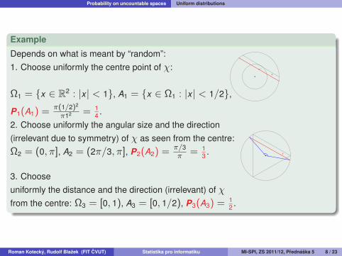
Example
Depends on what is meant by “random”:1. Choose uniformly the centre point of χ:
•χ
• x
1
Ω1 = x ∈ R2 : |x| < 1, A1 = x ∈ Ω1 : |x| < 1/2,P1(A1) = π(1/2)2
π12 = 14 .
2. Choose uniformly the angular size and the direction(irrelevant due to symmetry) of χ as seen from the centre:
•χ
1
Ω2 = (0, π], A2 = (2π/3, π], P2(A2) = π/3π = 1
3 .
3. Chooseuniformly the distance and the direction (irrelevant) of χfrom the centre: Ω3 = [0, 1), A3 = [0, 1/2), P3(A3) = 1
2 .
Roman Kotecky, Rudolf Blazek (FIT CVUT) Statistika pro informatiku MI-SPI, ZS 2011/12, Prednaska 5 8 / 23
Probability on uncountable spaces Properties of probabilities
As before (subaditivity, monotonicity, inclusion-exclusion,. . . ). In addition:
Theorem
Consider a probability P on (Ω,F) and a sequence of events A1,A2, · · · ∈ F .Thenσ-continuity: If either An ↑ A (i.e., A1 ⊂ A2 ⊂ . . . and A = ∪n≥1An)or An ↓ A (A1 ⊃ A2 ⊃ . . . and A = ∩n≥1An), then limn→∞ P(An) = P(A).
Proof.
An ↑ A: P(A) = P(∪n≥1(An \ An−1)) =∑
n≥1 P(An \ An−1) =
limn→∞∑n
k=1 P(Ak \ Ak−1) = limn→∞ P(An).
Roman Kotecky, Rudolf Blazek (FIT CVUT) Statistika pro informatiku MI-SPI, ZS 2011/12, Prednaska 5 9 / 23
Probability on uncountable spaces Properties of probabilities
Application for a repeated coin toss
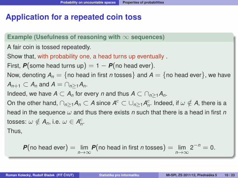
Example (Usefulness of reasoning with∞ sequences)
A fair coin is tossed repeatedly.Show that, with probability one, a head turns up eventually .First, P(some head turns up) = 1− P(no head ever).Now, denoting An = no head in first n tosses and A = no head ever, we haveAn+1 ⊂ An and A = ∩n≥1An.Indeed, we have A ⊂ An for every n and thus A ⊂ ∩n≥1An.On the other hand, ∩n≥1An ⊂ A since Ac ⊂ ∪n≥1Ac
n. Indeed, if ω /∈ A, there is ahead in the sequence ω and thus there exists n such that there is a head in first ntosses: ω /∈ An, i.e. ω ∈ Ac
n.Thus,
P(no head ever) = limn→∞
P(no head in first n tosses) = limn→∞
2−n = 0.
Roman Kotecky, Rudolf Blazek (FIT CVUT) Statistika pro informatiku MI-SPI, ZS 2011/12, Prednaska 5 10 / 23
Continuous random variables Density of a random variable
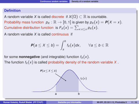
Definition
A random variable X is called discrete if X(Ω) ⊂ R is countable.Probability mass function pX : R→ [0, 1] is given by pX (x) = P(X = x).Cumulative distribution function is FX (x) =
∑x:x≤x pX (x).
A random variable X is called continuous if
P(a ≤ X ≤ b) =
∫ b
afX (x)dx, ∀a ≤ b ∈ R
for some nonnegative (and integrable) function fX (x).The function fX (x) is called probability density of the random variable X .
ba
P(a≤ X ≤ b)
fX (x)
Roman Kotecky, Rudolf Blazek (FIT CVUT) Statistika pro informatiku MI-SPI, ZS 2011/12, Prednaska 5 11 / 23
Continuous random variables Cumulative distribution function
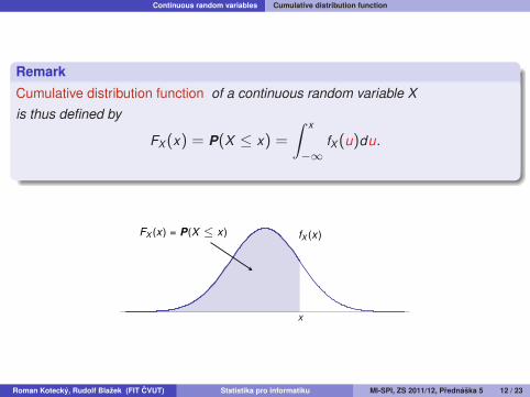
Remark
Cumulative distribution function of a continuous random variable Xis thus defined by
FX (x) = P(X ≤ x) =
∫ x
−∞fX (u)du.
FX (x) = P(X ≤ x) fX (x)
x
Roman Kotecky, Rudolf Blazek (FIT CVUT) Statistika pro informatiku MI-SPI, ZS 2011/12, Prednaska 5 12 / 23
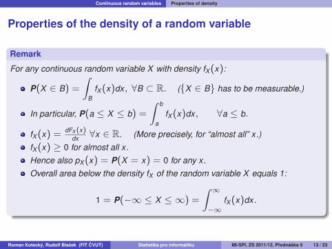
Continuous random variables Properties of density
Properties of the density of a random variable
Remark
For any continuous random variable X with density fX (x):
P(X ∈ B) =
∫B
fX (x)dx, ∀B ⊂ R. (X ∈ B has to be measurable.)
In particular, P(a ≤ X ≤ b) =
∫ b
afX (x)dx, ∀a ≤ b.
fX (x) = dFX (x)dx ∀x ∈ R. (More precisely, for “almost all” x.)
fX (x) ≥ 0 for almost all x.Hence also pX (x) = P(X = x) = 0 for any x.Overall area below the density fX of the random variable X equals 1:
1 = P(−∞ ≤ X ≤ ∞) =
∫ ∞−∞
fX (x)dx.
Roman Kotecky, Rudolf Blazek (FIT CVUT) Statistika pro informatiku MI-SPI, ZS 2011/12, Prednaska 5 13 / 23
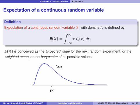
Continuous random variables Expectation
Expectation of a continuous random variable
Definition
Expectation of a continuous random variable X with density fX is defined by
E(X) =
∫ ∞−∞
x fX (x) dx.
E(X) is conceived as the Expected value for the next random experiment, or theweighted mean, or the barycenter of all possible values.
fX (x)
EX
Roman Kotecky, Rudolf Blazek (FIT CVUT) Statistika pro informatiku MI-SPI, ZS 2011/12, Prednaska 5 14 / 23
Continuous random variables Variance and general moments of the random variable
Variance of a continuous random variable
Definice
Consider a continuous random variable X with density fX .
Expectation of a function g(X) is defined by
E(g(X)) =
∫ ∞−∞
g(x) fX (x) dx.
Variance of X is defined by Rozptyl
var(X) = E[(X − E(X))2] =
∫ ∞−∞
(x − E(X))2 fX (x) dx.
We conceive var(X) as a mean quadratic deviation from the mean value (i.e. fromthe barycenter).
Roman Kotecky, Rudolf Blazek (FIT CVUT) Statistika pro informatiku MI-SPI, ZS 2011/12, Prednaska 5 15 / 23
Continuous random variables Variance and general moments of the random variable
General moments of a continuous random variable
Definice
Consider a continuous random variable X with density fX .
the k -th moment of X is defined by
mk = E(X k ) =
∫ ∞−∞
xk fX (x) dx, k = 1, 2, ...
the k -th central moment of X is defined by
σk = E((X − E(X))k ) = E((X − m1)k ) =
∫ ∞−∞
(x − m1)k fX (x) dx.
The variance var(X) = σ2 is often denoted as σ2 or σ2X with σ called the standard
deviation . smerodatna odchylka
Roman Kotecky, Rudolf Blazek (FIT CVUT) Statistika pro informatiku MI-SPI, ZS 2011/12, Prednaska 5 16 / 23
Examples of continuous random variables Uniform distribution
Uniform distribution
Example
Random variable X has the uniform distribution on the interval [a, b], if its density is
fX (x) =
1
b − a, for a ≤ x ≤ b
0, otherwise.
ba
fX (x)
Notation: X ∼ Unif(a, b) (Rovnomerne = Uniform)
Roman Kotecky, Rudolf Blazek (FIT CVUT) Statistika pro informatiku MI-SPI, ZS 2011/12, Prednaska 5 17 / 23
Examples of continuous random variables Uniform distribution
Example (continuation)
If X ∼ Unif(a, b) , then
E(X) =
∫ ∞−∞
x fX (x) dx =
∫ b
ax
1
b − adx
=1
b − a· 1
2x2
∣∣∣∣ba
=1
b − a· b2 − a2
2
=a + b
2.
ba
fX (x)
EX =a + b
2
Roman Kotecky, Rudolf Blazek (FIT CVUT) Statistika pro informatiku MI-SPI, ZS 2011/12, Prednaska 5 18 / 23
Examples of continuous random variables Uniform distribution
Example (continuation)
var(X) = E(X 2)− (E(X))2. For X ∼ Unif(a, b) , we get
E(X 2) =
∫ ∞−∞
x2 fX (x) dx =
∫ b
ax2 1
b − adx
=1
b − a· 1
3x3
∣∣∣∣ba
=b3 − a3
3(b − a)
=a2 + ab + b2
3.
Hence var(X) = E(X 2)− (E(X))2 =a2 + ab + b2
3− (a + b)2
4
=(b − a)2
12
Roman Kotecky, Rudolf Blazek (FIT CVUT) Statistika pro informatiku MI-SPI, ZS 2011/12, Prednaska 5 19 / 23
Examples of continuous random variables Uniform distribution
Example (continuation)
Summarizing, for a random variable with the uniform distribution:
E(X) =a + b
2, var(X) =
(b − a)2
12.
Roman Kotecky, Rudolf Blazek (FIT CVUT) Statistika pro informatiku MI-SPI, ZS 2011/12, Prednaska 5 20 / 23
Examples of continuous random variables Exponential distribution
Exponential distributionExample
A random variable X has an exponential distribution with parameter λ, if its densityis (for some λ > 0)
fX (x) =
λe−λx , for x ≥ 0
0, otherwise.
Notation: X ∼ Exp(λ) (λ > 0 is the parameter of the distribution)
1 2 3 4 5 6
12
1
2
λ=2
λ=1λ=1/2
Roman Kotecky, Rudolf Blazek (FIT CVUT) Statistika pro informatiku MI-SPI, ZS 2011/12, Prednaska 5 21 / 23
Examples of continuous random variables Exponential distribution
Example (continuation)
The expectation of X ∼ Exp(λ) is computed by the integration by part∫u v ′ = u v −
∫u′ v : per partes, po castech
E(X) =
∫ ∞−∞
x fX (x) dx =
∫ ∞0
x λe−λx dx
(u = x; u′ = 1); (v ′ = λe−λx ; v = −e−λx )
= (−x e−λx )∣∣∣∞0
+
∫ ∞0
e−λx dx
= 0− e−λx
λ
∣∣∣∣∞0
=1
λ
Roman Kotecky, Rudolf Blazek (FIT CVUT) Statistika pro informatiku MI-SPI, ZS 2011/12, Prednaska 5 22 / 23
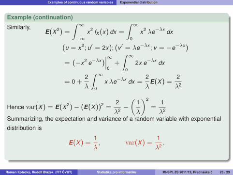
Examples of continuous random variables Exponential distribution
Example (continuation)
Similarly,E(X 2) =
∫ ∞−∞
x2 fX (x) dx =
∫ ∞0
x2 λe−λx dx
(u = x2; u′ = 2x); (v ′ = λe−λx ; v = −e−λx )
= (−x2 e−λx )∣∣∣∞0
+
∫ ∞0
2x e−λx dx
= 0 +2
λ
∫ ∞0
x λe−λx dx =2
λE(X) =
2
λ2
Hence var(X) = E(X 2)− (E(X))2 =2
λ2−(
1
λ
)2
=1
λ2
Summarizing, the expectation and variance of a random variable with exponentialdistribution is
E(X) =1
λ, var(X) =
1
λ2.
Roman Kotecky, Rudolf Blazek (FIT CVUT) Statistika pro informatiku MI-SPI, ZS 2011/12, Prednaska 5 23 / 23