118
TECHNICAL UNIVERSITY OF OSTRAVA FACULTY OF MECHANICAL ENGINEERING BASIC PRINCIPLES OF AUTOMATIC CONTROL Antonín Víteček, Miluše Vítečková, Lenka Landryová Ostrava 2012

TECHNICAL UNIVERSITY OF OSTRAVA
FACULTY OF MECHANICAL ENGINEERING
BASIC PRINCIPLES OF AUTOMATIC CONTROL
Antonín Víteček, Miluše Vítečková, Lenka Landryová
Ostrava 2012

Lektor: Prof. Ing. Zora Jančíková, CSc.
Copyright ©: Prof. Ing. Antonín Víteček, CSc., Dr.h.c.
Prof. Ing. Miluše Vítečková, CSc.
Doc. Ing. Lenka Landryová, CSc.
Basic Principles of Automatic Control
ISBN 978-80-248-4062-8

PREFACE
The major mission of this textbook is to highlight the importance of basic
principles of an automatic control by covering the most important areas from
analog automatic control, digital control, and two- and three-position control.
Hopefully, this textbook will stimulate new ideas by giving the reader basic
points of view of control system theory as well as appreciation of its use and
adaptability into complex systems.
The contents of this textbook originate in many texts and papers written by
the authors on their own, as well as hours of working on their approaches to the
basic methodology and experience with teaching it to students of control
engineering.
Since the textbook is concerned with the basic concepts of automatic
control, therefore the textbook does not have any given references itself. For
deepening your knowledge and extending your study materials the authors
recommend the references mentioned below for further reading:
DORF, R.C. – BISHOP, R. Modern Control Systems (12th ed.). Prentice-Hall,
Upper Saddle River, New Jersey 2011
FRANKLIN, G.F. – POWELL, J.D. – EMAMI-NAEINI, A. Feedback Control of
Dynamic Systems (4th ed.). Prentice-Hall, Upper Saddle River, New Jersey
2002
THE authors thank Prof. Ing. Zora Jančíková, CSc. for her valuable
suggestions.
Many key control techniques in use today have been founded on the very
basic principles of the past and we must not forget those ingenious individuals
of old who solved control problems with truly original solutions. The textbook
would like to point out these ideas which blended into our technologies and are
now taken for granted not only by students interested in control engineering.
Good technical ideas are precious and need to be respected by properly obeying
the basics when developing modern technological systems. If you enjoy reading
the book then the authors’ efforts were worthwhile.

CONTENT
1 Introduction 5
2 Mathematical Models 13
2.1 Linear Mathematical Models 15
2.2 Block Diagram Algebra 26
2.3 Linearization 29
3 Feedback Control Systems 32
3.1 Controllers 32
3.2 Plants 41
3.3 Control System Stability 49
4 Control System Synthesis 61
4.1 Process Control Performance 61
4.2 Controller Tuning 78
5 Digital Controllers 97
6 Two- and Three-position Controllers 102
7 Conclusion 109
8 References 110
Appendices
1 Laplace Transform – basic relations and properties 112
2 Laplace Transform – correspondences 114

5
1 INTRODUCTION
We meet with “control” or “drive” every day and all the time. The word
“control” is used in common cases, but the word “drive” is often used to mean
manual control. We drive (ride) a bicycle, a motorcycle, a car, etc. In these
cases, it is a manual control. An example of the simplified control of a car is
shown in Fig. 1.1. A driver tries to keep a desired path that is a desired lateral
displacement w(t) on the right side of the road with a steering wheel angle u(t)
regardless of disturbances v(t), i.e. current car velocity, the road condition and
its behavior (slopes, bends, zigzag bends etc.). The effect of his driving is the
true lateral displacement from the middle of the right side of the road y(t), see
Fig. 1.2.
Fig. 1.1 – Control of car on a road
Fig. 1.2 – Courses of a current y(t) and desired w(t) car displacement from the
middle of the right side of the road
The driver evaluates the current lateral displacement y(t) and by suitably
turning the steering wheel with angle u(t) he tries to minimize the difference
0)()()( tytwte (1.1)
which can be written in the equivalent form
)()( twty (1.2)
The relations (1.1) or (1.2) equivalently express the control objective.
Driver Car on road
Desired lateral
displacement
)(tw
Steering
wheel angle
)(tu
Current lateral
displacement
)(ty
Disturbance
)(tv
Road
)(ty
)(tw

6
We deal with automatic control so often that we do not perceive it. There
are controls for an iron´s temperature, the water temperature and level control in
the washing machine, the refrigerator and freezer temperature control, the room
temperature control, etc. in our homes.
Iron temperature control is shown in Fig. 1.3. The controlling device is
made from a bimetal strip, which bends when heated and the strip's bending
measures the current temperature of a heating body y(t). When this temperature
is lower than the adjusted desired temperature w(t), then the bimetal strip
switches on the heating body and it is supplied by a voltage u(t) (mostly 230 V).
When reaching the desired temperature )()( twty , the bimetal strip switches
off the heating body and it begins to cool down. After decreasing the heating
body temperature y(t) below the desired temperature w(t), the bimetal strip
switches on again. This process repeats.
Fig. 1.3 – Iron temperature control
In this case the disturbances v(t) can be e.g. the different moisture and
temperature of laundry. If the disturbances v(t) are constant, then the heating
and cooling processes are periodic.
It is obvious that in this case the bimetal strip fulfills these conditions (1.1)
or equivalently (1.2). The bimetal strip of an iron is one of the simplest
controlling devices. Therefore it operates in two states “switch-on” and “switch-
off”, it is called an“ON-OFF” controller or two-position controller.
There are different control systems in the present-day radio and television
sets, e.g. the automatic volume control, the automatic frequency control, voltage
and current stabilization, automatic brightness control, etc. Nowadays every
compact camera contains automatic focusing, automatic image stabilization, the
automatic white balancing, an automatic aperture and shutter setting, the
automatic tracking of an object, etc.
Very complex automatic control systems are especially used in automobile,
aviation, rocket and military technology.
Both control systems in Figs 1.1 and 1.2 can be generally presented by a
block diagram in Figs 1.4 and 1.5, where in the first case (Fig. 1.1) the
controller is implemented by a driver – a man (human) and in the second case
Bimetal
strip
Heating
body
)(tw
Supply
voltage
)(tu
Current
temperature
)(ty
Disturbances
)(tv Desired
temperatur
e

7
(Fig. 1.2) the controller is implemented by the bimetal strip – an automatic two-
position controller.
It is obvious that the sensor (measuring device) must be accurate and fast
and that is why its behavior is very often neglected or added to a plant or
process (controlled device). The control cannot be more accurate than the
sensor's accuracy is. Similarly, the behavior of an actuator (actuating device)
is added to a plant or to a controller (the controlling device) and a comparative
element is set apart in a separate summing node (a comparison device). The
disturbances are often aggregated into one or two selected disturbances. Then
the closed-loop control system or the feedback control system can be
obtained, where the desired output w(t) is the desired or reference variable, the
current controlled output y(t) is the controlled variable, the controller output
u(t) is the control, actuating or manipulated variable, the summing node
output e(t) is the control error, the aggregated disturbances v1(t) and v2(t) are
the disturbance variables.
Fig. 1.4 – General control system
Fig. 1.5 – Closed-loop control system
Controller +
comparison Plant
Desired
output
Current
controlled
output
Disturbances
Actuator
Sensor
Controller Plant )(tw
)(te )(tu
)(1 tv )(2 tv
)(ty

8
Negative feedback is very important, because determination of the control
error e(t) wasn’t enabled and the controller could not hold the demand (1.1) or
(1.2).
The demand (1.1) or (1.2) is called a control objective. Two controller
tasks follow from it. The first task is tracking a desired variable by the
controlled variable – the servo problem (set-point tracking), and the second
task is the rejection of the disturbances – the regulatory problem. The rejection
of a disturbance which is caused in the input of a process/plant is the most
frequent problem considered in the second case.
An open-loop control system or the feedforward control system can be
used in some simple cases, when the disturbances are negligible or they have
not influenced a control process. They are mostly very simple logical systems,
e.g. the traffic control, the washing machine etc. A traffic control is shown in
Fig. 1.6). The traffic light sequence and switching (green, amber, red) are
preprogrammed in accordance with the expected traffic flow depending on the
time of day and the kind of day (working day, holiday etc.). A simplified block
diagram of an open-loop system is shown in Fig. 1.7.
The behavior of both open-loop and closed-loop control systems is
explained below.
Fig. 1.6 – Traffic Flow Control
Fig. 1.7 – Open-loop control system
For example, consider the simple control systems in Fig. 1.8, where a
controller's behavior is expressed by the gain 0PK and a plant by the gain
01 k too.
We can perform an analysis of both open-loop (Fig. 1.8a) and closed-loop
(Fig. 1.8b) control systems
Controller Switching
time
setting Switch
Traffic
lights Crossing
Plant Desired
traffic
flow
Current
traffic
flow
Controller Plant )(tw
)(tu )(ty

9
a)
b)
Fig. 1.8 – A control system: a) open-loop structure, b) closed-loop structure
a) Open-loop control system (Fig. 1.8a)
In accordance with Fig. 1.8a we can write
)()()(1
tvtwkKtyP
(1.3)
On condition that the disturbance v(t) doesn’t cause a problem to an open-
loop control system, i.e. v(t) = 0, it is
1
1)()(
kKtwtyP (1.4)
which follows from the control objective (1.2).
If the disturbance v(t) ≠ 0, it will cause a problem to an open-loop control
system (Fig. 1.8a) and at the same time (1.4) will hold, then there can be
obtained
)()()( tvtwty (1.5)
We can see that the open-loop control system is unable to reject the
disturbance v(t), i.e. its influence on the controlled variable y(t).
If the behavior of a plant changes or is known with an accuracy 1k then
(1.5) has the form
)()(1)()()(1
1
1
11 tvtwk
ktvtw
k
kkty
(1.6)
From (1.6) it is obvious that the changes of a plant (uncertainty) 1k
fully come out on the controlled variable y(t).
For example, for k1 =1 and 5.0/11 kk (50 %) there is obtained
)()()5.01()( tvtwty
)(tw PK 1k
)(tu
)(tv )(ty
)(te
PK 1k
)(tw )(tu
)(tv )(ty

10
We can see that the change of the plant behavior and the disturbance fully
come out on the controlled variable. It is obvious that the open-loop structure is
suitable only for cases when the plant behavior is invariant and disturbances are
negligible.
b) Closed-loop control system (Fig. 1.8b)
We can write on the basis of Fig. 1.8b
)()]()([)(1
tvtytwkKtyP
)(1
1)(
11
1)(
1
1
tvkK
tw
kK
tyP
P
(1.7)
From (1.7) for
1
or kKKPP
(1.8)
relation
)()( twty (1.9)
is obtained.
We can see that for the sufficient high controller gain KP or the product
KPk1 the control objective (1.2) holds for a plant with an arbitrary finite gain k1
and at the same time the negative influence of a disturbance v(t) on a controlled
variable y(t) will be rejected. The same conclusion holds for plant changes or
uncertainties expressed by an increment of plant gain 1k :
)(
11
1)(
1
1
1
1)(
1
1
1
1
1
1
tv
k
kkK
tw
k
kkK
ty
P
P
(1.10)
If conditions (1.8) are fulfilled then (1.9) is obtained again.
For example, for KP = 100, k1 = 1 and 5.0/11 kk (50 %) there is obtained
on the basis of (1.10)
)(0097.0
0033.00099.0)(
0097.0
0033.09901.0)( tvtwty
We can see that the control objective (1.2)
)()( twty
holds with an accuracy better than 2 % even for a relatively small value of a
controller gain KP = 100 and for ± 50 % changes of plant behavior, i.e. its gain
k1. At the same time the negative influence of a disturbance v(t) is reduced to
less than 2 % as well.

11
A closed-loop control system enables superior control considerably more
than the open-loop control system. It is caused by the existence of the negative
feedback, which is a necessary condition not only for high-quality control but
for any meaningful activity of living beings and thus for a man. Living isn’t
possible without the existence of negative feedback.
It is very important that the high controller's gain KP occurs in the forward
path (branch).
A closed-loop control system even works out the non-linear plant. In Fig.
1.9 there is a control system with a non-linear plant, which is described by a
non-linear function
)()]([)( tvtufty (1.11)
Fig. 1.9 – A closed-loop control system with a non-linear plant
In accordance with Fig. 1.9, we can write
)()()()()()( tetwtytytwte (1.12)
PPK
tvtyf
K
tute
)]()([)()(
1
(1.13)
After substituting (1.13) in (1.12) there is obtained
PK
tvtyftwty
)]()([)()(
1
(1.14)
It is obvious that the relation holds
)()( twtyKP
We can see again that for a satisfactory high controller gain KP the control
objective (1.2) is available even for a non-linear plant and for the negative
influence of the disturbance (1.11).
At the end of this chapter the general system in Fig. 1.10 is considered. We
can symbolically describe the system by a following relation
tSuty
where S is an operator, which symbolically expresses the system’s behavior.
)(tw PK )]([ tuf
)(tu
)(tv )(ty
)(te
12
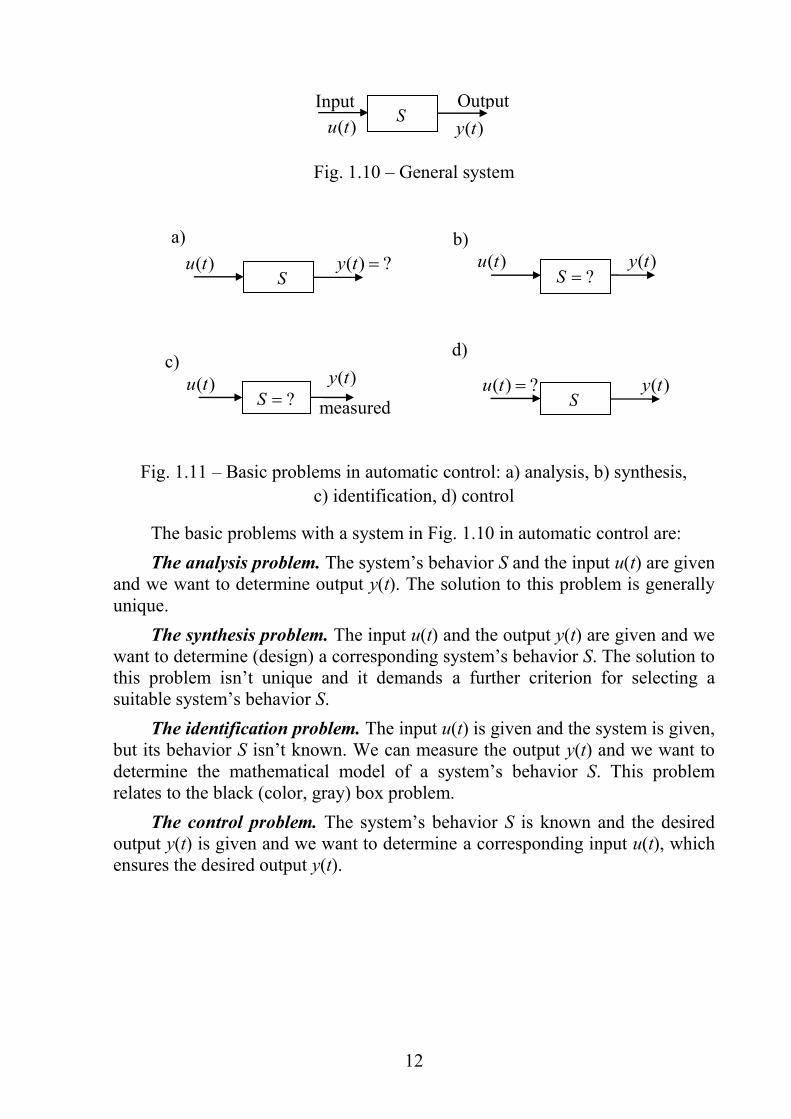
Fig. 1.10 – General system
Fig. 1.11 – Basic problems in automatic control: a) analysis, b) synthesis,
c) identification, d) control
The basic problems with a system in Fig. 1.10 in automatic control are:
The analysis problem. The system’s behavior S and the input u(t) are given
and we want to determine output y(t). The solution to this problem is generally
unique.
The synthesis problem. The input u(t) and the output y(t) are given and we
want to determine (design) a corresponding system’s behavior S. The solution to
this problem isn’t unique and it demands a further criterion for selecting a
suitable system’s behavior S.
The identification problem. The input u(t) is given and the system is given,
but its behavior S isn’t known. We can measure the output y(t) and we want to
determine the mathematical model of a system’s behavior S. This problem
relates to the black (color, gray) box problem.
The control problem. The system’s behavior S is known and the desired
output y(t) is given and we want to determine a corresponding input u(t), which
ensures the desired output y(t).
S ?)( tu )(ty
d)
?S )(tu )(ty
c)
measured
?S )(tu )(ty
b)
S )(tu ?)( ty
a)
S Input Output
)(tu )(ty

13
2 MATHEMATICAL MODELS OF SYSTEMS
We will consider the SISO (single-input single-output) system (Fig. 2.1).
Fig. 2.1 – Block representation of the SISO system
The dependence of a system output y(t) on its input u(t) expresses its static
and dynamic behavior. The time changes on a system input are called the action
or excitation and a corresponding system output time changes are called
reaction or response. A real, existing system has to hold the physical
realizability condition or the causality condition, which means that the
reaction – consequence cannot precede the action – cause.
The control systems are analyzed on their mathematical models. An
analogy is employed, which keeps the most important behavior of original
systems. If there is no difference between the original system and its
mathematical model behaviour and it does not cause any confusion, then a
mathematical model is called the original system. The input time functions are
called – inputs, input signals or input variables and similarly the output time
functions are called – outputs, output signals or output variables.
A mathematical model of the SISO system has often a form of a
differential equation in a time domain
0)](),(,),(),(),(,),([)()(
tutututytytygmn (2.1)
with initial conditions
)1(
0
)1(
00
)1(
0
)1(
00
)0(,,)0(,)0(
)0(,,)0(,)0(
mm
nn
uuuuuu
yyyyyy
(2.2)
mjt
tutututu
nit
tytytyty
j
jj
i
ii
,,2,1;d
)(d)(),()(
,,2,1;d
)(d)(),()(
)()1(
)()1(
(2.3)
where u(t) is an input variable, y(t) – an output variable, n – an order of a
differential equation and at the same time the order of an original system, g – is
generally a non-linear function.
If a mathematical model (2.1) satisfies the inequality
System
m
Input Output
)(tu )(ty

14
mn (2.4)
then the mathematical model is strongly physically realizable.
For
mn (2.5)
it satisfies only a weak physical realizability condition and for
mn (2.6)
the mathematical model isn’t physically realizable, i.e. a mathematical model
similar to this doesn’t correspond to any real existing system.
If on the basis of a differential equation (2.1) for
)(lim
,,2,1;0)(lim
)(lim
,,2,1;0)(lim
)(
)(
tuu
mjtu
tyy
nity
t
j
t
t
i
t
(2.7)
an equation can be obtained
)(ufy (2.8)
then this equation describes the static characteristic of a given model and, at
the same time, the original system (Fig. 2.2).
Fig. 2.2 – Non-linear static characteristic
A static characteristic expresses the dependency between an output y and
input u variables in a steady state.
The course of an output y(t) or input u(t) variables between two steady
states is called a transient process.
If in the equation (2.1) the derivatives (2.3) don’t arise, i.e..
0)](),([ tutyg or 0),( uyg (2.9)
u
y
)(ufy
0

15
then a mathematical model (2.9) describes a static system. The derivatives (2.3)
are basic attributes for dynamic behaviors, and therefore a differential equation
(2.1) describes a dynamic system.
2.1 Linear Mathematical Models
The linear models create a very important class of mathematical models.
Their most important behavior is linearity. The linearity of a dynamic system in
Fig. 2.1 can be expressed by two partial behaviors:
additivity (superposition):
)()()()()()(
)()(2121
22
11tytytutu
tytu
tytu
(2.10a)
homogeneity
)()(,)()( taytautytu (2.10b)
Both partial behaviors (2.10a) and (2.10b) can be expressed together
)()()()()()(
)()(22112211
22
11tyatyatuatua
tytu
tytu
(2.11)
where a, a1, a2 are any constants; u(t), u1(t), u2(t) – the input variables; y(t), y1(t),
y2(t) – the output variables.
The linearity of a dynamic system means that a weighting sum of output
variables corresponds to a weighting sum of input variables.
Another very important behavior of linear dynamic models (systems) is:
every local behavior of a linear dynamic system is at the same time its global
behavior.
A linear SISO system can be described in the time domain by a linear
differential equation with constant coefficients (with lumped parameters)
)()()()()()( 01
)(
01
)(tubtubtubtyatyatya
m
m
n
n (2.12)
with initial conditions
)1(
0
)1(
00 )0(,,)0(,)0(
nn
yyyyyy (2.13a)
)1(
0
)1(
00 )0(,,)0(,)0(
mm
uuuuuu (2.13b)
A static characteristic of a linear dynamic system is a straight line, which
goes through a co-ordinate´s origin (Fig. 2.3). It can be obtained simply from a
differential equation (2.12) for (2.7)
0),()( 0
0
0 atua
bty (2.14)
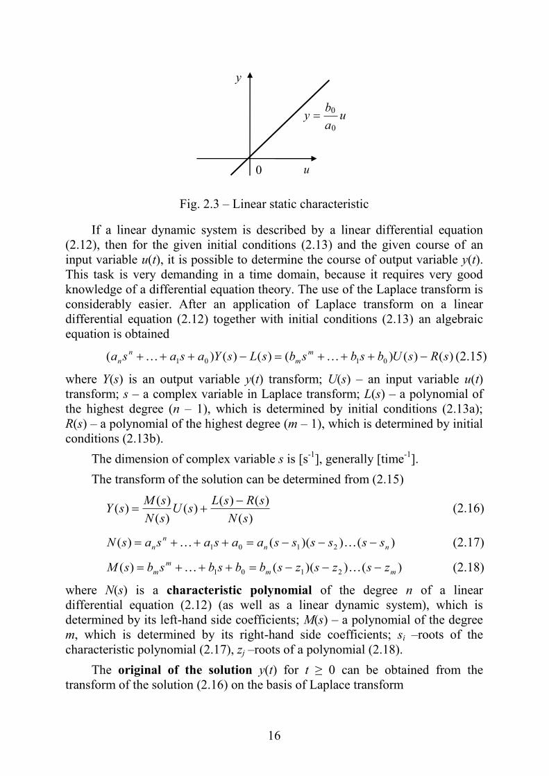
16
Fig. 2.3 – Linear static characteristic
If a linear dynamic system is described by a linear differential equation
(2.12), then for the given initial conditions (2.13) and the given course of an
input variable u(t), it is possible to determine the course of output variable y(t).
This task is very demanding in a time domain, because it requires very good
knowledge of a differential equation theory. The use of the Laplace transform is
considerably easier. After an application of Laplace transform on a linear
differential equation (2.12) together with initial conditions (2.13) an algebraic
equation is obtained
)()()()()()( 0101 sRsUbsbsbsLsYasasam
m
n
n (2.15)
where Y(s) is an output variable y(t) transform; U(s) – an input variable u(t)
transform; s – a complex variable in Laplace transform; L(s) – a polynomial of
the highest degree (n – 1), which is determined by initial conditions (2.13a);
R(s) – a polynomial of the highest degree (m – 1), which is determined by initial
conditions (2.13b).
The dimension of complex variable s is [s-1
], generally [time-1
].
The transform of the solution can be determined from (2.15)
)(
)()()(
)(
)()(
sN
sRsLsU
sN
sMsY
(2.16)
)())(()( 2101 nn
n
n ssssssaasasasN (2.17)
)())(()( 2101 mm
m
m zszszsbbsbsbsM (2.18)
where N(s) is a characteristic polynomial of the degree n of a linear
differential equation (2.12) (as well as a linear dynamic system), which is
determined by its left-hand side coefficients; M(s) – a polynomial of the degree
m, which is determined by its right-hand side coefficients; si –roots of the
characteristic polynomial (2.17), zj –roots of a polynomial (2.18).
The original of the solution y(t) for t ≥ 0 can be obtained from the
transform of the solution (2.16) on the basis of Laplace transform
u
y
ua
by
0
0
0

17
)(L)(1
sYty
(2.19)
The procedure is shown in Fig. 2.4.
The first part of the solution (2.16) is a transform of the response to an
input variable u(t), the second part of the solution (2.16) is the response to initial
conditions (2.13).
On the assumption that initial conditions are zeros, i.e.
0)(and0)( sRsL
the transform of the solution has a form
)()()( sUsGsY (2.20)
where the expression
)(
)(
)(
)()(
01
01
sN
sM
asasa
bsbsb
sU
sYsG
n
n
m
m
(2.21a)
is the transfer function of a linear dynamic system.
Fig. 2.4 – Solving a differential equation by the Laplace transform
The physical realizability conditions are given by relations (2.4) – (2.6).
Differential
equation
+
initial
conditions
L
Difficult
solution
Easy
solution
Original
of
solution
Transform
of solution -1L
Transforms Originals
Time domain Complex variable domain
Algebraic
equation

18
A transfer function (2.21a) expresses a mathematical model of a given
linear dynamic system for zero initial conditions in a complex variable domain
and can be presented by the block diagram in Fig. 2.5.
Fig. 2.5 – Block diagram of a system
For the following text zero initial conditions are supposed.
A transfer function (2.21a) can be written by means of linear dynamic
system poles si (i = 1, 2,…, n) and zeros zj (j = 1, 2,…, m)
)())((
)())((
)(
)()(
21
21
nn
mm
ssssssa
zszszsb
sU
sYsG
(2.21b)
A static characteristic of a linear dynamic system can be easily obtained
from its transfer function ( 00 a )
usGys
)(lim0
(2.22)
For a given course of the input variable u(t) a corresponding course of a
system response, i.e. the output variable y(t) can be determined in accordance
with the scheme
)(L)(
)()()(
)(L)(
1-sYty
sUsGsY
tusU
(2.23)
For a linear dynamic system the responses to the unit (Dirac) impulse
(Fig. 2.6)
0,1d)(,0for
0for0)(
ttt
tt (2.24a)
1)(L t (2.24b)
and the unit (Heaviside) step (Fig. 2.7)
0for0
0for1)(
t
tt (2.25a)
s
t1
)(L (2.25b)
are very important.
)(sG
)(sU )(sY

19
Fig. 2.6 – Unit impulse: a) undelayed, b) delayed
Fig. 2.7 – Unit step: a) undelayed, b) delayed
A linear dynamic system response to the unit impulse can be obtained on
the basis of (2.23) and (2.24b)
)()(L)(L)(-1-1
tgsGsYty (2.26)
The time function g(t) is the original of a transfer function G(s). It is called
the (unit) impulse response (Fig. 2.8).
t 0
1 )(t
t 0
1 )( dTt
dT
)a )b
t 0
1
)(t
t 0
1
)( dTt
dT
)a )b
20
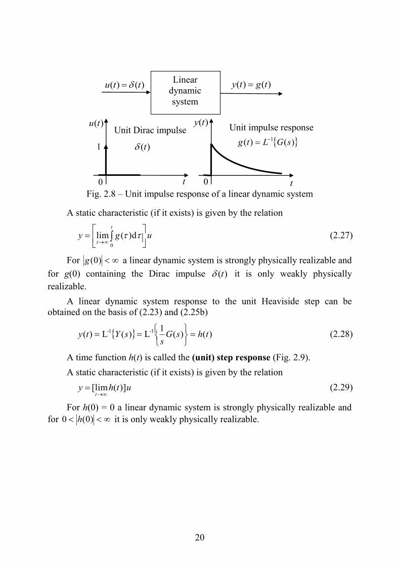
Fig. 2.8 – Unit impulse response of a linear dynamic system
A static characteristic (if it exists) is given by the relation
ugyt
t
0
d)(lim (2.27)
For )0(g a linear dynamic system is strongly physically realizable and
for g(0) containing the Dirac impulse )(t it is only weakly physically
realizable.
A linear dynamic system response to the unit Heaviside step can be
obtained on the basis of (2.23) and (2.25b)
)()(1
L)(L)(1-1-
thsGs
sYty
(2.28)
A time function h(t) is called the (unit) step response (Fig. 2.9).
A static characteristic (if it exists) is given by the relation
uthyt
)](lim[
(2.29)
For h(0) = 0 a linear dynamic system is strongly physically realizable and
for )0(0 h it is only weakly physically realizable.
Unit impulse response
Linear
dynamic
system
)()( ttu )()( tgty
0 t
1
)(tu
)(t
Unit Dirac impulse )(ty
)()(1
sGLtg
t 0

21
Fig. 2.9 – Unit step response of a linear dynamic system
The use of a generalized derivative is advantageous. It is defined by the
relations
)(lim)(lim
)()()(
txtx
tttxtx
ii tttti
iiior
(2.30)
where ti is the discontinuity points of the first kind with the steps Δi, )(txor – the
ordinary derivative, which is determined out of the discontinuity points.
On use of the generalized derivative (2.30) it is possible to write
t
tt
tt
0
d)()(d
)(d)(
(2.31)
t
gtht
thtg
0
d)()(d
)(d)( (2.32)
)(1
)()()( sGs
sHssHsG (2.33)
A mathematical model of a linear dynamic system in a state space has the
form (Fig. 2.10)
0)0(),()()( xxbAxx tutt – the state equation (2.34a)
)()()( tduttyT
xc – the output equation (2.34b)
where A is the square system matrix (n x n), b – the column input vector (n x 1),
cT – the row output vector (1 x n), d – the transfer constant, x(t) – the vector of
Linear
dynamic
system
)()( ttu )()( thty
0 t
1
)(tu )(t
Unit
Heaviside
step )(ty
Unit step response
s
sGLth
)()(
1
t 0
)(h

22
the state variables.
Fig. 2.10 – Block diagram of a SISO state space model
For d = 0 a mathematical model (2.34) satisfies the strong physical
condition and for d ≠ 0 only the weak physical realizability condition.
If a mathematical model (2.34) fulfills the controllability condition
0],,,det[],,,rank[11
bAAbbbAAbb
nnn (2.35)
and the observability condition
0])(,,,det[])(,,,rank[11
cAcAccAcAc
nTTnTTn (2.36)
then on the assumption that the initial conditions are zeros, on the basis of the
Laplace transform from (2.34) the transfer function can be determined
dssU
sYsG
sdUssY
sUsssT
T
bAIc
Xc
bAXX1
)()(
)()(
)()()(
)()()( (2.37)
where rank is a matrix rank, det – a determinant of the square matrix.
The relation (2.37) for practical use is not suitable, because it demands an
inversion of the functional matrix. Considerably preferable is the following
relation
ds
ss
sU
sYsG
T
)det(
)det()det(
)(
)()(
AI
AIbcAI (2.38)
A characteristic polynomial of a linear dynamic system with a
mathematical model (2.37) is given in accordance with (2.38)
)())((
)det()(
21
01
1
1
n
n
n
n
ssssss
asasasssN
AI (2.39)
where si are the eigenvalues of the matrix A.
It is obvious that the poles si of a linear dynamic system are given by the
eigenvalues of a square system matrix A.
b
Tc
A
0x
)(tx
)(ty u(t)
d

23
A static characteristic (if it exists) can be determined from a transfer
function (2.37) or (2.38) on the basis of (2.22).
On the assumption of zero initial conditions and fulfillment of the
controllability (2.35) and observability (2.36) conditions a transfer function
(2.37) or (2.38) is determined uniquely. A transformation of the transfer
function in a state space model is more complicated and non-unique. A state
space model of a linear dynamic system can have many different forms. It
depends on the choice of the state variables x(t) = [x1(t), x2(t),…, xn(t)]T. These
variables are “internal” variables, and therefore a state space model is often
called the internal model in contrast to the previous mathematical models,
which are called the external models.
0
0
φ ω( )
A( )ωIm
Re
0
ω
A(0)
0
0
π
2
π
2
π
ω
A(0)
A( )ω
ω = 0
ω
ω =
φ ω( )
a)b)
c)
G(j )ω
Fig. 2.11 – Frequency responses: a) polar plot, b) magnitude frequency
response, c) phase frequency response
A description of the linear dynamic system in the frequency domain is
very important. This description is based on the frequency transfer function,
which can be obtained from a transfer function G(s) by replacement of the
complex variable s with “complex frequency” jω, i.e.
01
01
j j)j(
j)j()()j(
aaa
bbbsGG
n
n
m
m
s
(2.40)
)(j)(jmod)( GGA (2.41a)

24
)(jarg)( G (2.41b)
where ω is the angular frequency or pulsation, 1j – the imaginary unit,
A(ω) – the modulus or magnitude of the frequency transfer function, φ(ω) –
the phase or phase-angle of the frequency transfer function.
The dimension of an angular frequency ω is the same as the dimension of a
complex variable s, i.e. [s-1
] or generally [time-1
], but for the reason to make a
distinction of the “ordinary” frequency with unit [s-1
] and the name Hz from an
angular frequency, the unit [rad.s-1
] is very often used.
0
φ ω ( )
[rad]
L( )
[dB]
ω
ω [s ] -1 1
0
ω [s ] -1 1
20
40
-20
0,01 0,1 10 100 1000
0,01 0,1 10 100 1000
π
2
π
2
π
d)
e)
Fig. 2.11 – Frequency responses: d) Bode magnitude plot, e) Bode phase plot
Mapping of a frequency transfer function to the angular frequency in a
complex plane from ω = 0 to ω = ∞ is called a polar plot or frequency
response (Fig. 2.11a). A selected mapping of the modulus (magnitude) A(ω)
and the phase φ(ω) from ω = 0 to ω = ∞ is called the magnitude frequency
response (Fig. 2.11b) and the phase frequency response (Fig. 2.11c). For
)(log20)( AL (2.41c)

25
Bode plots are obtained, i.e. Bode magnitude plot (Fig. 2.11d) and Bode phase
plot (Fig. 2.11e). L(ω) is the logarithmic modulus or logarithmic magnitude
(gain) [dB] of a frequency transfer function (2.40). For Bode plots the
approximation is used on the basis of the line sections and asymptotical lines,
i.e. (Fig. 3.5).
The frequency transfer function is very important for practice, because for
every angular frequency ω it expresses the magnitude (amplitude) A(ω) and the
phase φ(ω) of the steady-state harmonic response to the harmonic input with a
unit amplitude and a zero phase. It means that the frequency response can be
obtained experimentally, and therefore it can be used for the experimental
identification (Fig. 2.12).
Fig. 2.12 – Interpretation of a frequency response of a linear dynamic system
The physical realizability conditions are given by relations (2.4) – (2.6). In
case of a frequency transfer function (2.40) they have a very visual physical
interpretation. Since a frequency transfer function G(jω) describes the
transmission of a harmonic signal through a linear dynamic system for different
angular frequencies ω, it is obvious that the real linear dynamic system cannot
transmit a signal with infinity angular frequency, and this is why it must hold for
mathematical models of the physically realizable linear dynamic systems
mn
L
A
G
)(lim
0)(lim
0)(jlim
Linear dynamic system
ttu sin)( )](sin[)()( tAty
0 t
1
)(ty
tt
T
2)(
t 0
t
2T
)(A
2T
)(tu

26
It is a strong realizability condition. For the steady-state 0 t
holds, and therefore the static characteristic is given
0,)](jlim[ 00
auGy
(2.42)
2.2 Block Diagram Algebra
A great advantage of the description of the linear dynamic systems by the
transfer functions is the possibility to use the block diagrams. Every linear
dynamic system is presented by a block with its inscribed transfer function (Fig.
2.13a), the addition or subtraction of the variables (signals) are presented by the
summing nodes (Fig. 2.13b) and the variable (signal) branching is presented by
the information node (Fig. 2.13c).
U s( )G s( )
Y s( )
a) b)U s1( )
U s2( )
U s3( )
Y s( ) Y s( )
c) Y s( )
Y s( )
Y s( )
Fig. 2.13 – Representation: a) a linear dynamic system by a block, b) variable
addition or subtraction by a summing node, c) variable branching by an
information node
For a block in Fig. 2.13a it holds
)()()( sUsGsY
and for the summing node in Fig. 2.13b
)()()()( 321 sUsUsUsY .
Only one output from the summing node can go out.
The filled segment of the summing node expresses the minus sign. Besides
the filled segment the sign “-“ is often used too.
The function of an information node is obvious.
On the basis of the blocks and on the summing and information nodes very
complicated block diagrams can be created, which can always be reduced into
three basic block interconnections: serial (cascade), parallel and feedback.
27
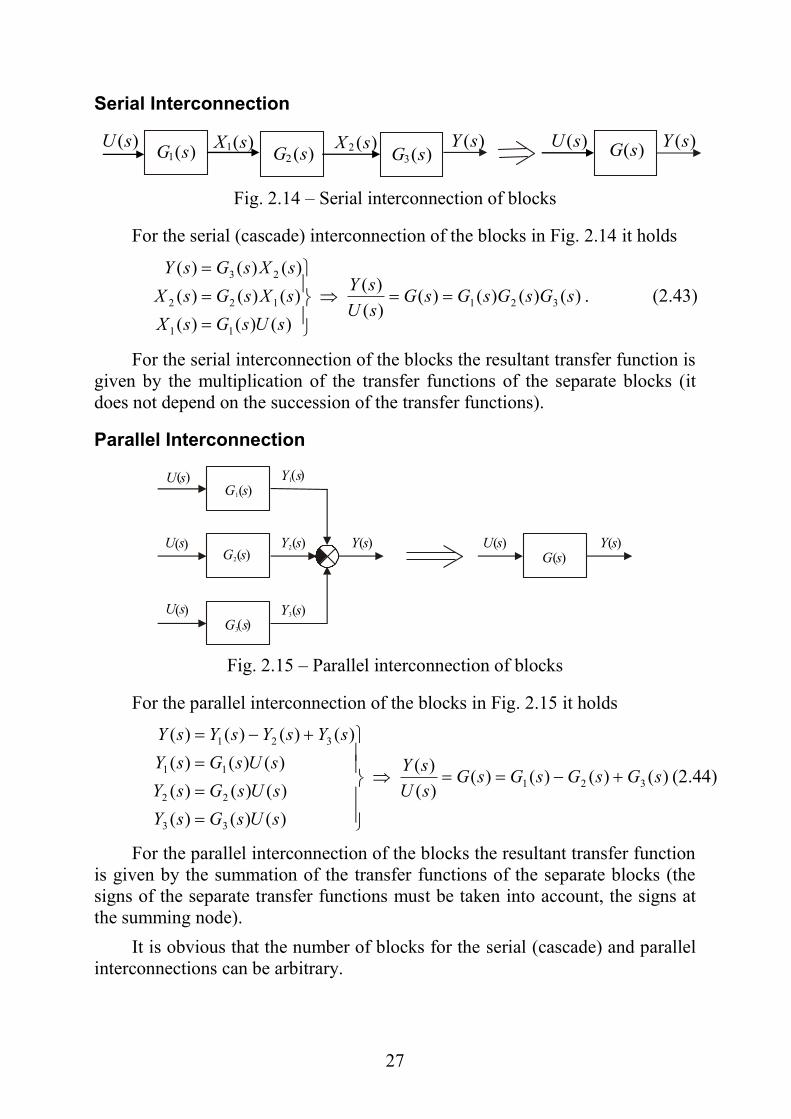
Serial Interconnection
Fig. 2.14 – Serial interconnection of blocks
For the serial (cascade) interconnection of the blocks in Fig. 2.14 it holds
)()()()()(
)(
)()()(
)()()(
)()()(
321
11
122
23
sGsGsGsGsU
sY
sUsGsX
sXsGsX
sXsGsY
. (2.43)
For the serial interconnection of the blocks the resultant transfer function is
given by the multiplication of the transfer functions of the separate blocks (it
does not depend on the succession of the transfer functions).
Parallel Interconnection
G s1( )Y s1( )
Y s( )G s3( )
U s( )G s( )
Y s( )Y s2( )
G s3( )Y s3( )
U s( )
U s( )
U s( )
G s2( )
Fig. 2.15 – Parallel interconnection of blocks
For the parallel interconnection of the blocks in Fig. 2.15 it holds
)()()()()(
)(
)()()(
)()()(
)()()(
)()()()(
321
33
22
11
321
sGsGsGsGsU
sY
sUsGsY
sUsGsY
sUsGsY
sYsYsYsY
(2.44)
For the parallel interconnection of the blocks the resultant transfer function
is given by the summation of the transfer functions of the separate blocks (the
signs of the separate transfer functions must be taken into account, the signs at
the summing node).
It is obvious that the number of blocks for the serial (cascade) and parallel
interconnections can be arbitrary.
)(1 sX
)(sU
)(1 sG
)(sY
)(2 sG
)(sG
)(sY
)(2 sX
)(3 sG
)(sU

28
Feedback Interconnection
Fig. 2.16 – Feedback interconnection of blocks
The feedback interconnection of the blocks in Fig. 2.16 is very important,
because it is the ground for all theory of automatic control. For the feedback
interconnection of the blocks in Fig. 2.16 it holds
)()(1
)()(
)(
)(
)()()(
)()()(
)()()(
21
1
22
21
11
sGsG
sGsG
sU
sY
sYsGsX
sXsUsX
sXsGsY
(2.45)
For the feedback interconnection of the blocks the resultant transfer
function is given by the transfer function in the forward path (branch) divided
by the negative (in case of sign “+”) or the positive (in case of sign “-“) product
of the transfer function in the forward path and the transfer function in the
feedback path increased by one. The transfer function of the branch without the
block (a transfer function) is a unit.
If we know these three basic interconnections of the blocks we can reduce
any complicated block diagram. We can use the Tab. 2.1. For the reason of
simplicity the independent variable s is not often explicitly written in the block
diagrams.
If the block diagram contains more input and output variables, for every
output variable the input variables are successively considered. The input
variables, which are not considered, are supposed to be zero (they aren’t drawn).
The resultant transfer functions are given on the basis of the linearity principle
by the summation of the influence of the separate input variables. For the reason
of unity the resultant transfer function uses subscripts. The first subscript
indicates the input variable and the second subscript the output variable.
Forward path
)(sG )(sU )(sY
Feedback path
)(1 sG )(1 sX )(sY
)(2 sG
)(sU
)(2 sX

29
Tab. 2.1 – Basic Block Diagram Transformations
Moving an information node ahead of a block
GY
Y
U
G
Y
Y
UG
Moving an information node behind a block
YUG
U
YU
U
G
1
G
Moving a summing node behind a block
YG
U2
U1
Y
U2
U1G
1
G
Moving a summing node ahead of a block
YG
U2
U1
YG
U2
U1
G
Moving a block from a parallel interconnection
U Y
G2
G1
U YG2
G1
1
G2
Moving a block from a feedback interconnection
U Y
G2
G1
U YG2
G1
1
G2
2.3 Linearization
In the previous subchapters we considered that all real systems (elements,
plants, processes etc.) are linear. In reality all real systems are non-linear, i.e.

30
their static and dynamic behaviors can be non-linear. If the non-linear behavior
of a given dynamic system is not substantial, then its behavior can be described
for small variable changes in the surroundings of the operating point by a
linear mathematical model. The linear mathematical model for a given or
selected operating point can be obtained from a non-linear mathematical model
by the linearization.
There exist many different linearization methods. The simplest method
only linearizes the non-linear static characteristics by analytical or graphical
ways. The more complex methods use optimization of some criteria. The least
squares method and its different modifications are often used.
If a static mathematical model of a system has only one output variable y
and m input variables u1, u2,…, um, i.e.
),,,( 21 muuufy (2.46)
then it is suitable to use in the operating point
),,,( 020100 muuufy (2.47)
an approximation on the basis of the tangent plane
yyy 0ˆ (2.48)
where
mm ukukuky 2211 (2.49)
is an increment of the output variable, i.e. ∆y = y – y0; and ∆u1 = u1 – u10, ∆u2 =
u2 – u20,…, ∆um = um – um0 are the increments of the corresponding input
variables, and
002
2
01
1 ,,,m
mu
fk
u
fk
u
fk
(2.50)
are the partial derivatives determined in the operating point (2.47), and y is an
output variable in the absolute form, which was obtained after linearization.
From a geometrical interpretation for one input (Fig. 2.17) it follows that the
coefficient k1 is the angular coefficient of a tangent line.

31
y
u 1
y = f(u1)
y = k1u1
u 10
u1 = u1 – u10
0
y 0
y = y – y 0
α = 1 arctg(k1)
Operating point = new origin
of incremental coordinates
Fig. 2.17 – Geometrical interpretation of linearization by a tangent line for one
input
The linearization on the basis of the tangent plane can be only used in a
case that the partial derivatives (2.50) exist and they are continuous. After
linearization the new origin in incremental coordinates (variables) must be
regarded in the operating point (2.47), see Fig. 2.17.
It is obvious that the linearization on the basis of the tangent plane can
keep its quality only for the small surrounding of the operating point.
In case of the differential equations, e.g. for the derivative of the i order
with respect to time it holds
i
i
i
i
i
i
t
ty
t
tyy
t
ty
d
)(d
d
)]([d
d
)(d 0
(2.51)
because y0 = const.
If the linearized mathematical model is complex, then it is useful to divide
it into simpler relations (models), and to linearize these simpler relations and
then to determine the resultant linear relation by the substitution. The algebra of
a block diagram can be used to great advantage.

32
3 FEEDBACK CONTROL SYSTEMS
This chapter is devoted to a description and an analysis of a control system.
Conventional linear analog controllers and simple identification methods for
basic plants are presented. The verification of the stability of the control systems
is described.
3.1 Controllers
A control system in Fig. 3.1 is considered, where GC(s) is the controller
transfer function, GP(s) – the plant transfer function, GS(s) – the sensor transfer
function, GV(s) – the disturbance allocating transfer function, W(s) – the
transform of the desired (reference) variable w(t), E(s) – the transform of the
control error e(t), U(s) – the transform of the control (manipulated, actuating)
variable u(t), Y(s) – the transform of the controlled variable y(t).
Fig. 3.1 – Block diagram of a common control system
For the reason of simplicity in lieu of the term “transform of variable” we
will only use “variable”.
A sensor (measuring device) with a transfer function GS(s) must measure
precisely and fast, therefore we may suppose that in practical cases its transfer
function is unit, i.e.
1)( sGS (3.1)
The controlled variable Y(s) can be obtained from the sensor, that’s why a
sensor is very often assigned to the plant.
The transfer function GV(s) enables allocating the disturbance V(s) in any
place in a control system. Two most important cases are in Fig. 3.2.
If disturbance variables cannot be measured or they are uncertain, then they
are aggregated in a one disturbance variable V(s) and a disturbance is then
allocated in the least advantageous place of a control system. In this case, it is
the plant’s input of an integrating plant (Fig. 3.2a) and the plant’s output in the
case of a proportional plant (Fig. 3.2b).
)(sW )(sGC )(sGP
)(sGV
)(sGS
)(sE )(sY )(sU
)(sV

33
a) b)
Fig. 3.2 – Control system with disturbance: a) in the input of a plant, b) in the
output of a plant
As noted previously, with the assumption that the condition (3.1) holds (the
closed-loop control system with a unit feedback), the control objective for the
control system in Fig. 3.1 can be expressed in two equivalent forms.
The control objective in the form:
)()(ˆ)()( sWsYtwty (3.2)
In accordance with Fig. 3.1 and (3.1) for the controlled variable holds
)()()()()( sVsGsWsGsY vywy (3.3)
where
)()(1
)()()(
sGsG
sGsGsG
PC
PCwy
(3.4)
is the desired variable to the controlled variable transfer function or the closed-
loop transfer function (the control system transfer function) and
)()](1[)()(1
)()( sGsG
sGsG
sGsG
Vwy
PC
V
vy
(3.5)
is the disturbance variable to the controlled variable transfer function or the
disturbance transfer function.
It is obvious that for fulfillment of the control objective (3.2) for any
desired variable W(s) and any disturbance variable V(s) the conditions
1)( sGwy servo (tracking) problem (3.6)
and
0)( sGvy regulatory problem (3.7)
must hold.
The first condition for the closed-loop transfer function (3.6) expresses the
controller function, which consists in the following desired variable W(s) by the
controlled variable Y(s) – it is the servo or tracking problem. The second
)(sGC )(sGP )(sE
)(sY
)(sV
)(sW 1)( sGV
)(sW )(sGC )(sE )(sY
)(sGP
)(sV )()( sGsG PV

34
condition for the disturbance transfer function (3.7) expresses the controller
function, which consists in the disturbance V(s) rejection (attenuation) – it is the
regulatory problem.
The control objective in the form:
0)(ˆ0)( sEte (3.8)
In accordance with Fig. 3.1 and (3.1) for the control error holds
)()()()()( sVsGsWsGsE vewe (3.9)
where
)(1)()(1
1)( sG
sGsGsG
wy
PC
we
(3.10)
is the desired variable to the control error transfer function and
)()](1[)()(1
)()( sGsG
sGsG
sGsG
Vwy
PC
V
ve
(3.11)
is the disturbance variable to the control error transfer function.
It is obvious that for fulfillment of the control objective (3.8) for any
desired variable W(s) and any disturbance variable V(s) the conditions
0)( sGwe servo (tracking) problem (3.12)
and
0)( sGve regulatory problem (3.13)
must hold.
Similarly like in previous case, the first condition for the desired variable
to the control error transfer function (3.12) expresses the servo problem and the
second condition for the disturbance variable to the control error transfer
function (3.13) expresses the regulatory problem.
It is obvious that both formulations (3.2) and (3.8) of the control objective
are equivalent and therefore further we will use the control objective in the form
(3.2).
The controller will operate correctly if the conditions (3.6) and (3.7) [or
(3.12) and (3.13)] will hold at the same time. If the disturbance variable V(s) is
effected in the plant output (Fig. 3.2b) then both conditions are equivalent (it is
the most frequent case), i.e. if the condition (3.6) holds then automatically the
condition (3.7) holds. Therefore, in automatic control theory attention is devoted
to the closed-loop transfer function (3.4). The transfer functions (3.4), (3.5),
(3.10) and (3.11) are called the basic transfer functions of the control system.
35
In accordance with (3.4) for the frequency closed-loop transfer function
there can be written
1)j()j(
1
1
)j()j(1
)j()j()j(
PC
PC
PCwy
GG
GG
GGG (3.14)
and it is obvious that relations
1)(1)j(0)j(
)j(
sGG
G
Gwywy
P
C
(3.15)
or
1)(1)j()j()j( sGGGG wywyPC (3.16)
hold.
From (3.15) it follows that if the satisfactory high controller modulus will
be ensured
)j()j(mod)( CCC GGA , (3.17)
then the condition (3.6) will hold with adequate accuracy and for non-singular
GV(s) the condition (3.7) as well.
If the plant behavior expressed by the transfer function GP(s) is known then
it is easier to ensure the high modulus of the frequency open-loop transfer
function
)j()j()j()j(mod)( PCooo GGGGA (3.18)
see (3.16).
The high moduli AC(ω) or Ao(ω) must be ensured for the band of the
operating frequencies and at the same time for the stability and desired
performance of the control system. This is practical by a suitable controller
choice and its successive controller tuning.
The industrial controllers are made in different versions and modifications,
and therefore only basic structures and modifications of the commonly used
controllers will be presented.
Analog (continuous) conventional controllers are implemented as a
combination of three components (terms): proportional – P, integral – I and
derivative – D. The controller with all three components is called the
proportional plus integral plus derivative controller or the PID controller.
Its behavior can be described by the relation

36
t
teTe
TteK
D
t
teK
I
eK
P
teKtu D
t
I
PD
t
IPd
)(dd)(
1)(
d
)(dd)()()(
00
(3.19)
where KP, KI and KD are the proportional, integral and derivative component
weights, KP – the controller gain (the proportional component weight), TI – the
integral time, TD – the derivative time.
In industrial controllers the proportional band
%100
PKpp (3.20)
is often used.
The dimension of the proportional component weight KP, i.e. the controller
gain is given by the dimension of the control variable u(t) divided by the
dimension of the control error e(t). The time constants TI and TD have the
dimension of time [s]. The dimension of the integral component weight KI is
given by the dimension of KP divided by time and the dimension of the
derivative component weight KD is given by the product of the dimension of KP
and time.
The parameters KP, KI and KD or KP, TI and TD are adjustable controller
parameters. The task of controller tuning is to ensure the desired control
performance by suitable tuning (setting) of the adjustable controller parameters
for a given plant. Among the adjustable controller parameters the conversion
relations hold
DPD
I
PI TKK
T
KK , (3.21)
or
P
DD
I
PI
K
KT
K
KT , (3.22)
After using the Laplace transform on relation (3.19) the controller transfer
function
sTsT
KsKs
KK
sE
sUsG D
I
PDI
PC
11
)(
)()( (3.23)
is obtained.
In Fig. 3.3 there are drawn the courses of the moduli of the controller
components P, I and D. From Fig. 3.3 it follows that the integral component (I)
ensures the high value of the frequency transfer function modulus of the PID

37
controller for small angular frequencies and especially for the steady state
(ω = 0), the derivative component (D) for high angular frequencies and the
proportional component for all angular frequencies (mainly for medium
frequencies). In fact by a suitable choice of the particular components P, I and
D, i.e. by the suitable setting of the adjustable controller parameter KP, KI and
KD or KP, TI and TD it is possible to achieve a high modulus of the frequency
controller transfer function (3.17) or a high modulus of the frequency open-loop
transfer function (3.18), in order to fulfill the conditions (3.15) or (3.16).
0
I D
P
II
I
P
I
P
KK
T
K
T
K
j
j
DD
DPDP
KK
TKTK
j
j
PP KK
ω
)(CA
Fig. 3.3 – Dependence of partial controller components P, I and D of PID on
angular frequency
Tab. 3.1 – Conventional analog controller transfer functions
Type Transfer function )(sGC
1 P PK
2 I sTI
1
3 PI
sTK
I
P
11
4 PD sTK
DP1
5 PID
sTsT
KD
I
P
11
6 PIDi sTsT
K D
I
P
1
11

38
In industrial practice simpler controllers are often used. They are: the P
(proportional) controller, the I (integral) controller, the PI (proportional plus
integral) controller and PD (proportional plus derivative) controller. Their
transfer functions are in Tab. 3.1 (rows 1 – 5). The single D component is
unusable because it only reacts to the derivative )(te and therefore in a steady
state it causes a disconnection of the control system.
The block diagram of the PID controller with the transfer function (3.23) is
in Fig. 3.4a. From the Fig. 3.4a it follows that it has a parallel structure. The
adjustable parameters of this controller can be tuned independently. Therefore
this PID controller is without interaction (non-interacting).
a)
b)
Fig. 3.4 – Block diagram of a PID controller with a structure: a) parallel
(without interaction), b) serial (with interaction)
Sometimes the PID controller form with weights (3.23) is only considered
as a controller with a parallel structure and the PID controller form with the time
constants is considered as a standard form according to ISA (The International
Society of Automation formerly Instrument Society of America).
The PID controller can be implemented by the serial (cascade) structure
(Fig. 3.4b), which is described by relation
sT
sTsTKsT
sTKsG
I
DI
PD
I
PC
)1)(1(
PD
1
PI
11)(
(3.24)
)(sW
)(sY
sTD
PK
)(sE )(sU
sTI
1
)(sW )(sE )(sU PK
sTI
1 sTD )(sY

39
This relation may be transformed into a parallel structure (3.23)
)1
1
11()( s
T
TT
TT
s
T
TT
K
T
TTKsG
D
DI
DI
I
DI
P
I
DI
PC
(3.25)
From (3.25) it follows that the change of the integral time IT or derivative
DT time comes to change all values of the adjustable controller parameters KP,
TI and TD, which corresponds to the parallel structure, i.e. the interaction among
the adjustable controller parameters happens. Therefore the PID controller with
the serial structure is called the PID controller with interaction (interacting)
and it is marked like the PIDi controller (Tab. 3.1, row 6). Among the adjustable
controller parameters for the parallel and serial structure the following relations
hold
I
DDDIIPP
T
Ti
i
TTiTTiKK
1,,, (3.26)
I
DDDIIPP
T
TTTTTKK
4
1
2
1,,,
(3.27)
The coefficient i is called the interaction factor. Most of controller tuning
methods suppose the PID controller (without interaction) and therefore the
adjustable controller parameters PK , IT and DT of the PIDi controller (with
interaction) must be recounted for parameters KP, TI and TD on the basis of
(3.26).
For the PIDi controller in accordance with (3.27) the restriction
4
1
I
D
T
T (3.28)
there arises.
The approximate Bode plots of the PIDi controller [with interaction (3.24)]
are shown in Fig. 3.5.
If the condition (3.28) holds then the approximate Bode plots of the PID
controller [without interaction (3.23)] have the same courses as in Fig. 3.5, but
the relations (3.27) must be considered.
From Fig. 3.5 it follows again that the integral component ensures the high
value of the controller modulus for low angular frequencies firstly for steady
states, the derivative component for high angular frequencies and the
proportional component for all angular frequencies in the operating band. The
serial structure of the PIDi controller has some advantages. It can be simply

40
implemented by the serial interconnection of the PI and PD controllers [Fig.
3.4b and (3.24)] and therefore it is cheaply manufactured. For 0 DD TT both
structures are equivalent to the PI controller.
Fig. 3.5 – Bode plots of PIDi controller
From a theoretical point of view the derivative component has a positive
stabilizing effect on the control process, but from a practical point of view it has
very unpleasant behavior, which consists in the amplification of high frequency
noise and fast changes (Fig. 3.3 and 3.5). E.g. if the derivative component of the
PD or PID controllers
t
teTK
t
teK DPD
d
)(d
d
)(d (3.29)
processes the control error e(t), which contains harmonic noise with the
amplitude an and the angular frequency ωn
tate nn sin)(
then the derivative component (3.29) output is
]cosd
)(d[ ta
t
teK
nnnD (3.30)
where t
teKD
d
)(d is the useful part of the derivative component output and
taK nnnD cos is the parasitic part of the derivative component output.
2
0
0
]dB[
)(CL
PK log20
IT
1
DT
1
IT
1
DT
1 ]s[
1
]s[1
[rad]
)(C
2

41
It is obvious that for high angular frequencies ωn the parasitic part will
dominate over the useful part and then the output of the derivative component
can cause an incorrect controller function, thereby even over all the control
system. Hence the ideal derivative operation is practically unusable. For
attenuation of the parasitic part a filter of the derivative component is used. Its
transfer function is given
NsTs
N
TDD
1,
1
1
1
1
(3.31)
where N = 5 ÷ 20 or α = 0.05 ÷ 0.2.
The task of the filter is to attenuate the parasitic noise in the controlled
variable y(t). For α ≤ 0.1 the filter doesn’t have a principle effect on the resultant
controller behavior, therefore during controller tuning it isn’t considered. In
industrial controllers the filter (3.31) is often preset at a value α = 0.1 (N = 10).
The transfer function of the PID controller with the filter has the form
1
11)(
sT
sT
sTKsG
D
D
I
PC
(3.32)
A very unpleasant effect, which appears in controllers with the integral
component, is the windup. The windup is caused by limiting the control
variable, when the integration goes on and big overshoots arise. For windup
removal a special mechanism must be used – the antiwindup.
3.2 Plants
The mathematical models of the plants may have different forms. For the
linear plants the transfer functions with time constants are frequently used. The
time constants are marked so that inequalities
,2,1,0,1 iTT ii (3.33)
hold, i.e. the time constant with a lower subscript has a higher or the same value
than the time constant with a higher subscript.
The obtaining of the mathematical model of the real plant (object) is called
the identification. The identification can be analytical or experimental. The
practical identification methods lie between these two marginal cases. It is
always useful to find the approximate relations describing given plant in the
theoretical way and then experimentally to determine model parameters more
precisely. For better prepared analytical relations experimental measurements
are shorter and cheaper.

42
Every concrete plant demands a different identification method. Finding
the most suitable identification approach supposes some intuition and
experience.
Furthermore, some simpler experimental identification methods will be
shown, which use step responses. It is supposed that the courses of the step
responses are suitably prepared (filtered, smoothed etc.) and that all variables
are in incremental forms, i.e. the courses begin in the origin of coordinates.
Proportional non-oscillating plants
If the plant is non-oscillating and has the step response hP(t) as in Fig 3.6a
then the simplest identification method consists in the determination of the time
delay Tu = Td = Td1 and the time constant Tn = T1. The first order plus time delay
(FOPTD) plant transfer function has the form
sTP
d
sT
ksG 1e
1)(
1
1
(3.34)
a) b)
)(thP
t 0 Tu Tn
Tp
S
)(Ph
t 0 t0.33
S
)(Ph
t0.7
)(7.0 Ph
)(33.0 Ph
)(thP
Fig. 3.6 – FOPTD plant identification on the basis of:
a) time delay Tu = Td1 and time constant Tn = T1, b) times t0.33 and t0.7
The plant gain k1 for proportional plants for the unit step of the input
variable, i.e. Δu(t) = η(t) is given by the steady state in the step response
)(1 Phk (3.35)
because hP(0) = 0.
For general value of the step Δu(t) = Δu the plant gain k1 is given
u
hk P
Δ
)(1
(3.36)
The dimension of the plant gain k1 is given by the ratio of the dimension of
the output variable yP(t) = hP(t) to the dimension of the input variable Δu(t).

43
A very good mathematical model can be obtained by the Strejc method. It
is suitable for proportional non-oscillating plants. The approximate value of the
time delay dT must be determined at first and then on the basis of the times Tu
and Tn the ratio
n
du
T
TT
is computed and in Tab. 3.2 the nearest lower value of the ratio
n
diu
n
ddu
T
TT
T
TTT
Δ (3.37)
must be found and then the plant order i is determined. The plant transfer
function is given by the formula
sT
i
i
Sdi
sT
ksG
e
)1()( 1 (3.38)
where time delay is
dddi TTT Δ (3.39)
and Ti is determined from row 3 or 4 ( dT is the correction of the estimation
dT ).
Tab. 3.2 – Strejc method of experimental identification
i 1 2 3 4 5 6
n
diu
T
TT 0 0.104 0.218 0.319 0.410 0.493
i
diu
T
TT 0 0.282 0.805 1.425 2.100 2.811
i
n
T
T
1 2.718 3.695 4.463 5.119 5.699
If the times t0.33 and t0.7 (Fig. 3.6b) are used for the experimental
identification, then for the FOPTD plant (3.34) the formulas can be used
7.033.01
33.07.01
498.0498.1
245.1
ttT
ttT
d
(3.40)
For the second order plus time delay (SOPTD) plant with the transfer
function

44
sT
Sd
sT
ksG 2e
12
2
1
(3.41)
the formulas
7.033.02
33.07.02
937.0937.1
794.0
ttT
ttT
d
(3.42)
can be used.
The relation
)(
P
diih
STiT (3.43)
can be used for the approximate verification of the (3.34), (3.38) and (3.41),
where S is the complementary area over the step response hP(t), see Fig. 3.6.
The relations (3.40) were obtained analytically and the relations (3.42)
numerically from the correspondences of the original step response and the
approximate step response in the values hP(0) = 0, hP(t0.33) = 0.33hP(∞), hP(t0.7) =
0.7hP(∞) and hP(∞).
A very good approximation of the SOPTD plant with different time
constants T1 and T2 is given by the following formulas
sT
P
d
sTsT
ksG 2e
1121
1
(3.44)
where
2233.07.01
7.033.02
2
1
2
222
2
1
2
221
)(,794.0
937.0937.1
42
1,4
2
1
d
S
d
Th
SDttD
ttT
DDDTDDDT
(3.45)
In order to use the transfer function in the form (3.44), the inequality
D2 > 2D1, must hold otherwise the transfer function (3.41) must be used.
For fast conversion of the transfer function (3.38) on the simpler transfer
functions (3.34) and (3.41) in accordance with the scheme

45
sT
i
i
di
sT
e
1
1
(3.46)
sTd
sT1e
1
1
1
sTd
sT
2e1
12
2
on the basis of Tab. 3.3 can be used.
Tab. 3.3 – Table for fast transfer function conversion in accordance
with scheme (3.46)
sT
ii
di
sT
e
1
1
i 1 2 3 4 5 6
sTd
sT1e
1
1
1
iT
T1
1 1.568 1.980 2.320 2.615 2.881
i
did
T
TT 1
0 0.552 1.232 1.969 2.741 3.537
sTd
sT
2e1
12
2
iT
T2
0.638 1 1.263 1.480 1.668 1.838
i
did
T
TT 2
*
–0.352 0 0.535 1.153 1.821 2.523
* Applicable for Td1 > 0.352T1.
Tab. 3.3 was obtained numerically on condition that the values hP(0),
hP(t0.33), hP(t0.7) a hP(∞) of the original and the conversed step responses are the
same.
Non-oscillating integrating plants
The identification of the integral plus first order plus time delay (IFOPTD)
plants with the transfer function
sT
Pd
sTs
ksG 1e
)1()(
1
1
(3.47)
can be made on the basis of their step responses hP(t) in accordance with Fig.
3.7a. The dimension of the plant gain k1 is given by the ratio of the dimension of
the output variable yP(t) = hP(t) and the dimensions of the input variable Δu(t)

46
and time.
All previous methods for identification of the proportional plants can be
used for identification of the simple integrating plants if we use the impulse
response (the derivative of the step response)
)(d
)(dtg
t
thP
P
in lieu of the step response hP(t).
a) b)
)(thP
t 0
k1
)( 1 uk
Td1+T1
1 Td1
t 0
k1
)( 1 uk
T1 Td1
t
t h t g
P P
d
) ( d ) (
Fig. 3.7 – Identification of integrating plants on the basis of:
a) step response hP(t), b) impulse response gP(t)
It is shown in Fig. 3.7b for the IFOPTD plant with the transfer function
(3.47).
If the step of the input variable isn’t a unit, i.e. Δu(t) ≠ η(t) but it is Δu(t) =
Δu, then it is necessary to consider the values, which are in parentheses in Fig.
3.7.
Conversion of plant transfer functions
Some of the methods for the analysis and synthesis of control systems
demand that the plant transfer functions have specific forms. These forms can be
obtained by the simple transfer function conversion.
The conversion of the transfer function in the form (3.38) on the 1st or 2nd
order form can be made on the basis of scheme (3.46) and Tab. 3.3.
The simple conversions of the transfer functions without derivations are
given below. These conversions come from the equality of supplementary areas
over the step responses.

47
Proportional plants
a)
niTTTT
sTsT
k
sTsT
k
i
n
ii
n
ii
,3,2,,
1111
12
1
1
21
1
(3.48)
b)
niTTTT
sT
k
sTsT
k
i
n
iid
sT
n
ii
d
,3,2,,
e1
11
12
1
1
21
1
(3.49)
c)
niTTTTT
sTsT
k
sTsTsT
k
i
n
iid
sT
n
ii
d
,,4,3,,
e11
111
213
21
1
321
1
(3.50)
d)
niTTTT
sTsT
k
sTsTsT
k
i
n
iid
sT
n
ii
d
,,2,1,,
e12
112
01
00
22
0
1
100
22
0
1
(3.51)
Integrating plants
e)
11
1
1
1
sTs
k
sTs
kn
ii
,
n
iiTT
1
(3.52)

48
f)
sT
n
ii
d
s
k
sTs
k
e
1
1
1
1 ,
n
iid TT
1
(3.53)
g)
niTTTT
sTs
k
sTsTs
k
i
n
iid
sT
n
ii
d
,,3,2,,
e1
11
12
1
1
21
1
(3.54)
The use of a combination of the summary time constant T∑ and the
substitute time delay Td is advantageous.
If in the numerator of the plant transfer function stands up the binomials
si1 (3.55)
then each binomial can be substituted by the term
sie (3.56)
on condition that the resultant time delay will be non-negative.
The “half rule” is very simple and simultaneously effective.
On the assumption that the plant transfer function has a form with unstable
zeros
sT
ii
jj
Pd
sT
s
sG 0e)1(
)1(
)(0
0
(3.57)
0,0, 000,10 djii TTT
then on the basis of the “half rule” we can obtain
j
ji
idd TT
TTT
TT 03
020
0120
1012
,2
(3.58)
for the transfer function (3.34) or
j
ji
idd TT
TTT
TTTT 04
030
0230
2021012
,2
, (3.59)
for the transfer function (3.44).
The resultant time delay Td1 or Td2 must be always non-negative.

49
3.3 Control System Stability
Stability of the linear control system is defined as its ability to fix all
variables on finite values if input variables are fixed. The input variables are the
desired variable w(t) and all disturbance variables, which are often aggregated
into one disturbance variable v(t).
It is obvious that the following stability definition is equivalent. The linear
control system is stable if for any bounded input the output is always
bounded. It is so-called BIBO (bounded-input bounded-output) stability.
From both definitions it follows that stability is the characteristic behavior
of the given control system, which doesn’t depend on the inputs and outputs (it
doesn’t hold for non-linear systems).
Therefore the control system is fully described by the equation (3.3)
)()()()()( sVsGsWsGsY vywy
or (3.9)
)()()()()( sVsGsWsGsE vewe
it is obvious that stability is given by the term, which figures in all the basic
transfer functions, i.e. Gwy(s) and Gvy(s) or Gwe(s) and Gve(s). From relations
(3.4) and (3.5) or (3.10) and (3.11) it follows that this term is their denominator
)(
)(
)(
)()(
)(
)(1)(1)()(1
sN
sN
sN
sMsN
sN
sMsGsGsG
oo
oo
o
ooPC
(3.60)
where Go(s) is the open-loop transfer function of the control system (it is
generally given by the product of all transfer functions in the loop), No(s) – the
characteristic polynomial of the open-loop of the control system (the
denominator of the open-loop transfer function), Mo(s) – the polynomial of the
numerator of the open-loop transfer function.
The polynomial
)()()( sMsNsN oo (3.61)
is the characteristic polynomial of the control system and after its equating to
zero the characteristic equation of the control system
0)( sN
is obtained.
The characteristic polynomial (3.61) rises after its arrangement in the
denominators of all basic transfer functions of the control system, i.e. (3.4),
(3.5), (3.10) and (3.11) and therefore it is simultaneously the characteristic
polynomial of the relevant linear differential equation, which describes the
given control system.

50
A necessary and sufficient condition for (asymptotic) stability of the linear
differential equation and the corresponding linear dynamic system is that the
roots s1, s2,..., sn of the characteristic polynomial (or the characteristic equation)
)())(()( 2101 nn
n
n ssssssaasasasN (3.62)
have negative real parts, i.e. (see Fig. 3.8)
nisi
,,2,1for,0Re (3.63)
It is obvious that the conditions of the negativeness of the real parts of the
roots (i.e. poles) (3.63) of the characteristic polynomial of the control system
(3.61) [(3.62)] are the necessary and sufficient conditions for (asymptotic)
stability of the given linear control system.
Because the concept of the stability of the non-linear systems has a rather
different meaning, it is necessary in some cases when the necessary and
sufficient conditions hold to use a more precise concept of “asymptotic”
stability.
The complex roots, i.e. poles of the control system rise always in the
conjugate couple (i.e. in the symmetry of the real axis in the s-complex plane). It
is very important that the poles s1, s2,..., sn of the control system are at the same
time the poles of all of its basic transfer functions. It doesn’t hold for the zeros
of the basic transfer functions. The poles of the control system determine its
dynamic behavior.
The necessary and sufficient condition for stability (3.63) of the control
system can be obtained in another way.
Consider any basic transfer function of the control system, e.g.
)(
)()(
sN
sMsGwy (3.64)
and the desired variable transform
)(
)()(
sN
sMsW
w
w (3.65)
where M(s), Mw(s) and Nw(s) are the polynomials and N(s) is the characteristic
polynomial of the control system.
On condition that the characteristic polynomial of the control system N(s)
has the simple roots s1, s2,..., sn and the polynomial Nw(s) has the simple roots wp
wwsss ,,, 21 [p is the degree of the polynomial Nw(s)], the transform of the
controlled variable (response)
)(
)(
)(
)()()()(
sN
sM
sN
sMsWsGsY
w
wwy (3.66)

51
can be written in the form of the sum of the partial fractions
)()()(
)(
1
)(
1
sYsYss
B
ss
AsY ST
sY
p
jw
j
j
sY
n
i i
i
ST
(3.67)
where YT(s) is the transform of the transient response part, YS(s) – the transform
of the steady response part.
The original of the controlled variable y(t) can be obtained from (3.67) on
the basis of the Laplace transform
tsp
jj
n
i
ts
iST
wji BAtytyty ee)()()(
11
(3.68)
The constants Ai and Bj in the relations (3.67) and (3.68) generally depend
on the forms of the transfer function Gwy(s) and the desired variable transform
W(s), see (3.64) and (3.65).
The course of the transient part of the controlled variable yT(t) depends on
the roots of the characteristic polynomial of the control system, i.e. on its poles
and it is given as
n
i
ts
iT
iAty1
e)(
The course of the steady part of the controlled variable
tsp
jjS
wjBty e)(
1
is given by the course of the desired variable w(t).
Here by its steady course it is necessary to understand the given time
function, e.g. yS(t) = Bt, yS(t) = Bsinωt etc. in contrast to the steady (static) state,
e.g. yS(t) = yS = const.
From (3.68) it follows that for the bounded input variable – the desired
variable w(t) ( 0Re wjs for j = 1, 2,..., p) the output variable – the controlled
variable y(t) will be bounded if and only if its the transient part yT(t) will be
bounded, i.e. the condition (3.63) will hold. Therefore for the stable control
system the transient part yT(t) must vanish for t → ∞ , i.e.
0)(lim
tyT
t (3.69)
therefore for t → ∞
)()( tytyS
(3.70)
holds.
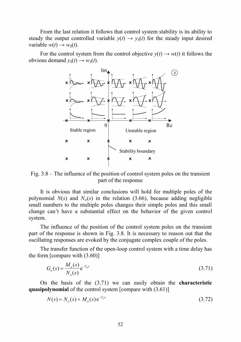
52
From the last relation it follows that control system stability is its ability to
steady the output controlled variable y(t) → yS(t) for the steady input desired
variable w(t) → wS(t).
For the control system from the control objective y(t) → w(t) it follows the
obvious demand yS(t) → wS(t).
Re 0
Im s
Stable region Unstable region
Stability boundary
Fig. 3.8 – The influence of the position of control system poles on the transient
part of the response
It is obvious that similar conclusions will hold for multiple poles of the
polynomial N(s) and Nw(s) in the relation (3.66), because adding negligible
small numbers to the multiple poles changes their simple poles and this small
change can’t have a substantial effect on the behavior of the given control
system.
The influence of the position of the control system poles on the transient
part of the response is shown in Fig. 3.8. It is necessary to reason out that the
oscillating responses are evoked by the conjugate complex couple of the poles.
The transfer function of the open-loop control system with a time delay has
the form [compare with (3.60)]
sT
o
oo
d
sN
sMsG
e
)(
)()( (3.71)
On the basis of the (3.71) we can easily obtain the characteristic
quasipolynomial of the control system [compare with (3.61)]
sT
oodsMsNsN
e)()()( (3.72)

53
The characteristic quasipolynomial (3.72) has an infinite number of roots,
i.e. the control system with the time delay has an infinite number of poles. That
is why the stability verification by the necessary and sufficient conditions (3.63)
by the direct computation isn’t real.
Control system stability is the only necessary condition for its proper
operation. For verification of control system stability different stability criteria
are used, which enable checking the fulfillment of inequalities (3.63) without
labored computation of all roots of the control system characteristic polynomial
or quasipolynomial N(s).
Furthermore, the three stability criteria are given without derivation:
Hurwitz, Mikhailov and Nyquist criteria.
Hurwitz stability criterion
The Hurwitz stability criterion is an algebraic criterion and therefore it isn’t
suitable for the control systems with a time delay (the exponential function isn’t
an algebraic function). It can be used only for approximate stability verification
in the case that the time delay will be substituted by its algebraic approximation.
The Hurwitz stability criterion can be formulated in the form:
„The linear control system with the characteristic polynomial
01)( asasasNn
n
is (asymptotic) stable [i.e. the conditions (3.63) hold] if and only if, when:
− all coefficients a0, a1,..., an exist and are positive (it is a necessary
stability condition formulated by Slovak technician A. Stodola)
− the main corner minors (subdeterminants) of the Hurwitz matrix
0
31
42
531
000
00
0
0
a
aa
aaa
aaa
nn
nnn
nnn
H (3.73)
H
n
nn
nn
n Haa
aaHaH ,,
2
31
2,11
are positive.“
Because the equality H1 = an–1, Hn = a0Hn–1 hold, it is enough to check only
the positiveness of H2, H3, ..., Hn–1. If some of the Hurwitz minors are zero, then
it determines the stability boundary. E.g. for a0 = 0 Hn = 0 one pole is zero
(it is the origin of the coordinates in the complex plane s). This case
characterizes the non-oscillating stability boundary. For Hn–1 = 0 two poles are
imaginary and conjugate (they are on the imaginary axes in symmetry by the

54
origin of the coordinates in the complex plane s). This case characterizes the
oscillating stability boundary, see Fig. 3.8.
If the Stodola necessary condition of the stability holds, then the simplified
Lineard – Chipart stability criterion can be used, which consists only in
checking of the positiveness of all odd or all even Hurwitz minors.
The disadvantage of the Hurwitz criterion is its high demandingness of
computation for n ≥ 5.
Mikhailov stability criterion
The Mikhailov stability criterion is a frequency criterion with a wide range
of use. Here only a simple formulation will be given, which is suitable for
control systems without a time delay.
The Mikhailov stability criterion uses the control system characteristic
polynomial N(s), from it after substituting s = jω the Mikhailov function
)(j)()()(jj
QPs
NNsNN
(3.74)
is obtained, where
4
4
2
20)(jRe)( aaaNN P (3.75a)
is the real part and
5
5
3
31)(jIm)( aaaNNQ (3.75b)
is the imaginary part of the Mikhailov function.
The Mikhailov stability criterion can be formulated in the form:
„The linear control system is (asymptotic) stable if and only if its
Mikhailov function (plot) N(jω) for 0 ≤ ω ≤ ∞ begins on the positive real axis
and successively passes through n quadrants in a positive direction
(anticlockwise).“

55
a)
Re 0
Im
a 0
n = 2
ω = 0
n = 3
n = 4
n = 1
)(jN
Stable control systems
ω
ω
ω
ω
b)
Re 0
Im
a 0
ω n = 2
ω = 0
n = 3 n = 4
n = 1
N (j ) ω
Unstable control systems
ω
ω
ω
Fig. 3.9 – Mikhailov plots for control systems:
a) stable, b) unstable
This formulation can be written in a form for changing the argument
(angle) of the Mikhailov function
2)(jarg
0
nN
(3.76)
where n is the characteristic polynomial N(s) degree.
The courses of the Mikhailov functions (plots) for the stable control
systems are in Fig. 3.9a and for unstable control systems in Fig. 3.9b.
The Mikhalov function can be employed for an analytical determination of
the ultimate (critical) angular frequency ωc and the ultimate (critical) controller
gain KPc or the ultimate (critical) controller integral time TIc.
Re 0
Im
a 0
ω n = 5
n = 3
N (j ) ω
ω
Non-oscillating stability boundary
Oscillating stability boundary
ω = 0
Fig. 3.10 – Mikhailov plots for control systems on the stability boundary
For this the equations

56
0 and 0 QP NN (3.77)
are used.
The ultimate parameters (ωc, KPc or TIc), more correctly their values, cause
that the control system is on a stability boundary, i.e. in the critical state
between stability and instability. In this case a slight change of these values
causes stability or instability of a given control system.
Nyquist stability criterion
The Nyquist stability criterion is a frequency criterion, which in contrast to
the Hurwitz and Mikhailov criteria uses the open-loop frequency transfer
function Go(jω). It is very general and it can be extended for unstable open-loop
control systems and even for non-linear control systems.
The control system in Fig. 3.11 is considered. It is obvious that when
oscillations arise with a constant amplitude and an angular frequency on the
stability boundary [for W(s) = V(s) = 0] it is necessary that oscillations in the
feedback path must be the same as oscillations in the forward path but with a
negative sign, see Fig. 3.11. It can be written in the transforms
1)(j1)( coo
GsG (3.78)
where Go(s) = GC(s)GP(s) is the open-loop transfer function (it is generally given
by the product of all transfer functions in the loop), ωc – the ultimate angular
frequency.
Fig. 3.11 – Control system on stability boundary
It is obvious that this conclusion can be made on condition that the open-
loop control system is stable (otherwise the stable oscillations in the control
loop wouldn’t be possible).
The relation (3.78) expresses the given control system condition for the
oscillating stability boundary. It can be obtained from the same denominators of
the basis transfer functions of the control systems [see e.g. (3.4), (3.5), (3.10)
and (3.11)], where the term 1 + Go(s) stands out. It is obvious that the critical
state arises when this term will be equal to zero, which corresponds with (3.78).
)(sGC )(sW
)(sGP )(sY
)(sV
)(sE
)(ty
t
)(te
t

57
The relation (3.78) expresses the fact that if the control system is on the
oscillating stability boundary, then the frequency response (polar plot) of the
open-loop control system comes through the point –1+j0 on the negative real
axis. This point is called the critical point. The frequency response of the open-
loop control system is called the Nyquist plot.
Furthermore, from the relation (3.78) and Fig. 3.14 it follows that if the
value e.g. Go(jωp) = –0.5 in lieu of Go(jωp) = Go(jωc) –1 was in it, the
oscillations would decrease (i.e. the control system is stable) and vice versa for
value e.g. Go(jωp) = –2 the oscillations would increase (the control system is
unstable).
The Nyquist stability criterion can be formulated in the form:
„The linear control system is (asymptotic) stable if and only if when the
frequency response of the stable open-loop control system, i.e. the Nyquist plot
Go(jω) for 0 doesn’t enclose the critical point –1+j0 on the negative
real axis.“
The main cases of the Nyquist plots Go(jω) are shown in Fig. 3.12. The
integrating elements in the forward path or feedback path (i.e. in the loop) from
the point of view of the Nyquist stability criterion aren’t considered as unstable
(they are in fact neutral elements). The number of these integrating elements q is
called the control system type.
In the case the integrating elements exist the decision about if that the
Nyquist plot encloses or doesn’t enclose the critical point –1+j0 must be made
in accordance with the Fig. 3.13.
Re 0
Im
ω =
q = 0
Go (j ω )
ω = 0
-1
Stable
On stability boundary
Unstable
Critical point
Fig. 3.12 – Nyquist plots Go(jω) for control system with q = 0
If the Nyquist plot Go(jω) for q = 2 has the course as in Fig. 3.13 then the
control system is conditionally stable, because the increasing or decreasing of
the Ao(ω) for the phase –π can cause the instability of the control system.

58
Above the geometrical form of the Nyquist stability was formulated. The
analytical formulation of the Nyquist stability criterion is also very useful. We
can write
1)( go
A (3.79)
)( po (3.80)
where ωg is the gain crossover angular frequency, ωp – the phase crossover
angular frequency.
For the oscillating stability boundary holds
pgc (3.81)
Now the Nyquist stability criterion can be written in different analytical
forms:
1)(jRe)(j popo
GG , 1)( poA (3.82)
)( go (3.83)
Re 0
Im
ω =
Go (j ω )
ω 0
-1
q = 2
q = 1
ω 0
Stable control systems
r
r
Fig. 3.13 – Nyquist plots Go(jω) for stable control systems with q = 1 and q = 2

59
Re 0
Im
g
G O (j ω )
ω 0
-1
q = 1
p
-1
1
1
)(1
po
A
Am
ω =
γ
)( go
Fig. 3.14 – Gain margin mA and phase margin γ
It is obvious that these simple analytical formulations hold for
nonconditionally stable control systems. For conditionally stable systems these
formulations can be easily extended.
On the basis of the angular frequencies ωg and ωp further important indices
can be defined (Fig. 3.14):
the gain margin
)(
1
po
AA
m
(3.84)
and the phase margin
)( go (3.85)
The gain margin mA expresses how many times the magnitude Ao(ωp) can
be increased (how many times the open-loop gain ko can be increased) in order
for the control system to reach the stability boundary. Similarly the phase
margin γ expresses how much the phase φo(ωg) (in the absolute value) can be
increased in order for the control system to reach the stability boundary.
Because the controller integral component brings the negative phase in the
open-loop of the control system (see Fig. 3.5), i.e. it decreases the phase margin
γ, therefore the controller integral component destabilizes (i.e. it deteriorates
the stability) the control system. On the other hand the controller derivative
component brings the positive phase in the open-loop of the control system (see
Fig. 3.5), i.e. it increases the phase margin γ, therefore the controller derivative
component stabilizes (i.e. improves the stability) the control system [of
course for suitable filtration, see e.g. (3.31 and 3.32)].

60
Regarding the controller gain KP, it is obvious that by its increasing it
simultaneously increases the open-loop gain ko and hence the gain margin is
decreased, therefore the controller proportional component destabilizes the
control system (it doesn’t hold for conditionally stable control systems).
Time delay is very dangerous for the control system stability. The
frequency transfer function of the time delay has the form
)(jje)(e)(j
AG dT
(3.86)
1)( A (3.87)
dT)( (3.88)
From the relations (3.86) – (3.88) it follows that the time delay doesn’t
change the modulus (magnitude) [see (3.87)] but linearly increases the negative
phase [see (3.88)], i.e. it decreases the phase margin γ. Therefore the time delay
always essentially destabilizes the control system.

61
4 CONTROL SYSTEM SYNTHESIS
The chapter is devoted to process control performance and the linear
control system synthesis, i.e. to controller choices and their tuning. Basic known
and new controller tuning methods are brought up. Some of them are also for
the digital controller.
4.1 Process Control Performance
The control objective expressed in two equivalent forms (3.2) and (3.8) or
by couple relations (3.6), (3.7) and (3.12), (3.13) [see as well (3.15), (3.16)] can
be held with a different process control performance and only on the condition
that a given control system is stable. It is obvious that process control
performance can be reviewed in: the time domain, the frequency domain and the
complex variable domain. Different criteria and indices can be used for it.
Time Domain
The time domain is very popular among the control system technicians and
designers because it enables the fast and intuitive evaluation of process control
performance on the basis of the step responses y(t) caused by the step changes
of the desired variable w(t) or the disturbance variable v(t). It is useful to
inscribe the responses with subscripts in accordance with the input variables.
For simultaneous actuating the desired variable w(t) and the disturbance
variable v(t) on the basis of the linearity principle it holds
)()()()()()()( sYsYsVsGsWsGsY vwvywy
)()()( tytyty vw (4.1)
where yw(t) is the response caused by the desired variable w(t) for v(t) = 0, yv(t)
– the response caused by the disturbance variable v(t) for w(t) = 0.
The typical control system oscillatory and non-oscillatory responses in
incremental variables (i.e. in increments from the operation point) are shown in
Figs 4.1 and 4.2. A very important conclusion comes from them. If the
disturbance variable v(t) influences the plant output then for the same input
steps the servo (setpoint) response and regulatory response are in principle the
same as well (the regulatory response is turned up and moved, see Figs 4.1 and
4.2). It is given by relation Gvy(s) = 1 – Gwy(s). The steady-state errors ev(∞) for
the control systems in Fig. 3.2 and the steps of the disturbance variable v(t) have
negative values, see Figs 4.2b and 4.4b and relation (3.11).
The servo and regulatory responses for the disturbance variable caused in
the plant output with the zero steady-state errors in Fig. 4.1 correspond to a case
when the open-loop contains at least one integrating element, i.e. the control

62
system type q ≥ 1. The integrating element (component) can be included in the
controller or in the plant.
Fig. 4.1 – Control system step responses in the case of zero steady-state errors:
a) servo (setpoint) responses, b) regulatory responses for disturbance variable in
the plant output
Fig. 4.2 – Control system step responses in case non-zero steady-state errors:
a) servo (setpoint) responses, b) regulatory responses for disturbance variable in
plant output
The servo and regulatory responses for the disturbance variable caused in
the plant output with non-zero steady-state errors in Fig. 4.2 correspond to the
case when the open-loop doesn’t contain any integrating element, i.e. the control
system type q = 0
If the disturbance variable v(t) influences the plant input (in Figs 4.3 and
4.4 the oscillating responses are only shown), then it is necessary to distinguish

63
the causes if the plant contains the integrating elements (it has an integrating
character) or doesn’t contain the integrating elements (it has a proportional
character).
Fig. 4.3 – Control system step responses for a controller with integral
component and proportional plant: a) servo (setpoint) response, b) regulatory
response for a disturbance variable in plant input
Fig. 4.4 – Control system step responses for a controller without an integral
component and integrating plant: a) servo (setpoint) response, b) regulatory
response for a disturbance variable in the plant input
If the plant has a proportional character and the controller contains the
integral component (e.g. I, PI, PID) then q = 1 and the steady-state errors are
zero, see Fig. 4.3. From Fig. 4.3 it follows that the regulatory response yv(t) is
often very well attenuated by the plant. It is caused by the filtration (inertia)
behavior of the plant. Therefore the controller can be tuned more aggressively,

64
i.e. it is possible to increase the controller gain KP or to decrease the integral
time TI.
If the plant has an integrating character (only one integrating element is
considered) then in the case of the use of the controllers without the integral
component (e.g. P, PD) the control system is type q = 1 but still for the
disturbance in the plant input the regulatory response will be with a non-zero
error, see Fig. 4.4b. For controllers with the integral component the steady-state
errors ew(∞) and ev(∞) will be zero for the input steps. In this case the control
system type q is 2.
The steady-state errors can be determined on the basis of the following
relations
)()()()()()()( sEsEsVsGsWsGsE vwvewe (4.2)
)(lim)(),(lim)(00
ssEessEe vs
vws
w
(4.3)
where ew(∞) is the steady-state error caused by the desired variable w(t), ev(∞) –
the steady-state error caused by the disturbance variable v(t).
The mentioned relations (4.2) and (4.3) generally hold for any changes of
the input variables w(t) and v(t), e.g. for the velocity or acceleration steps etc.
The steady-state errors can be decreased by increasing the controller gain
KP (in the case of the I controller by decreasing the integral time TI).
If the plant has an integrating character and the disturbance variable v(t)
causes in the plant input then it is necessary to reason it out in controller tuning.
By ensuring suitable behavior of the control system from the point of view
of the desired variable w(t), the corresponding behavior of the control system
from the point of view of the disturbance variable v(t) (for a disturbance caused
in the plant output it always holds) will be ensured in most cases too. Therefore
further the servo (tracking) problem is solved first of all and that is why the
subscripts w will not be mostly used.

65
Fig. 4.5 – Servo (setpoint) responses with marked control performance indices
In Fig. 4.5 two typical courses of the servo (setpoint) response are shown.
From the practical point of view the most important performance indices are:
the settling time tr and the relative overshoot
)(,)(
)(mm
m tyyy
yy
(4.4)
where ym is the maximum value of the controlled variable y(tm) (the first
maximum or peak), tm – the time of reaching the value ym (the peak time), y(∞) –
the steady state value of the controlled variable. The settling time is determined
by the time when the controlled variable y(t) gets in the band with a width 2Δ,
i.e. y(∞) Δ, where the control tolerance is given
05.001.0),( y (1 5) % (4.5)
The relative control tolerance δ mostly has a value 0.05 or 0.02.
For the settling time tr the relative control tolerance δ must be mentioned
otherwise it is supposed δ = 0.05 (5 %).
The case κ = 0 corresponds to a non-oscillating (aperiodic) control process,
which is used for processes where the overshoot can cause undesirable effects
(e.g. thermal and chemical processes, assembly robots and manipulators etc.).
For the non-oscillating control process, the minimum of the settling time is
demanded very often. This control process is called the marginal non-
oscillating control process.
For κ > 0 the control process is oscillating and faster then the non-
oscillating process. The time for reaching the value y(∞) is the rise time to. Very
often the rise time is defined like the time required for the response to go from
0.1y(∞) to 0.9y(∞).

66
The control process with the relative overshoot κ about 0.05 (5 %) is
acceptable for most plants. If the minimum of the settling time tr is
simultaneously ensured then this control process is regarded as practically
“optimal”. It is widely accepted everywhere that the small overshoot doesn’t
matter or is desirable, e.g. for the indicator measuring and recording devices (in
this case the small overshoot enables a faster interpolating of the indicator
position).
The integral criteria are very useful for the complex evaluating of the
control performance. The shade area in Fig. 4.6 expresses the so-called control
area.
It is obvious that the control area will be smaller and the control
performance will be higher. It is suitable to work with the control error e(t) =
w(t) – y(t) (see Figs 4.6b, c, d) on condition e(∞) = ew(∞) = 0. If e(∞) ≠ 0, then
in all relations for the integral criteria the term e(t) – e(∞) must be substituted in
lieu of e(t)
Integral of error (Fig. 4.6b)
min d)(0
tteI IE (4.6)
The integral of error IIE (IE = Integral of Error) is the simplest integral
criterion. It isn’t suitable for oscillating control processes, because IIE = 0 for the
control process on the oscillating stability boundary (the areas marked with
signs + and – are mutually subtracted). Its best advantage is that it can be easily
computed (see appendix)
0000
d)(de)(lim)(lim ttettesEIst
ssIE (4.7)
Integral of absolute error (Fig. 4.6c)
min d)(0
tteI IAE (4.8)
The integral of absolute error IIAE (IAE = Integral of Absolute Error)
removes the disadvantage of the previous integral criterion IIE (see Fig. 4.6c),
and therefore it is applicable for both non-oscillating and oscillating control
processes. It has a very unpleasant behavior and generally cannot be calculated
analytically but only numerically or by simulation.
It is obvious that the control area in Fig. 4.6a is (4.8) too.

67
Fig. 4.6 – Geometrical interpretation of integral criteria: a) control area,
b) integral of error IIE, c) integral of absolute error IIAE,
d) integral of squared error IISE
Integral of squared error (Fig. 4.6d)
min d)(0
2
tteI ISE (4.9)
The integral of squared error IISE (ISE = Integral of Squared Error)
removes the disadvantages of both previous integral criteria IIE and IIAE. It can
be used for non-oscillating and oscillating control processes and its value can be
calculated in an analytical way. It is very suitable in these cases when the

68
desired w(t) and the disturbance v(t) variables have a random character. Some
disadvantage of the integral of squared error consists in that the control process
is too oscillating.
For the control error transform
01
01
1
1)(asasa
bsbsbsE
n
n
n
n
(4.10)
can be computed:
10
2
0
21
aa
bIn ISE (4.11)
210
2
02
2
10
22
aaa
babaIn ISE
(4.12)
)(2
)2(3
302130
2
0323020
2
1
2
210
aaaaaa
baaaabbbbaaIn ISE
(4.13)
For higher degree n the formulas are very complex.
ITAE criterion
min d)(0
ttetI ITAE (4.14)
The ITAE criterion IITAE (ITAE = Integral of Time multiplied by Absolute
Error) contains the time and the error and therefore it simultaneously
minimalizes both the settling time and the error. This integral criterion is very
popular among technicians though its value can be determined generally by
simulation.
For the given control system type q and the characteristic polynomial N(s)
with degree n so-called standard forms of the control system transfer functions
were determined by simulation for minimum of the ITAE criterion.
Below are shown the standard forms only for q = 1, n = 2 and 3:
)4.1(4.1)(
4.1)(,2
2
2
2
22
2
ass
a
ass
asG
aass
asGn owy
(4.15)
)15.275.1(15.275.1)(
15.275.1)(,3
22
3
223
3
3223
3
aasss
a
saass
asG
asaass
asGn
o
wy
(4.16)

69
The parameter a matches the time scales of the original system and its
model in a standard form. From both transfer functions of the open-loop control
system Go(s) it follows that they contain one integrating element, i.e. q = 1.
Only the most important integral criteria were briefly described. By their
minimization the optimal values of the adjustable controller parameters can be
obtained. The minimization is generally done by simulation.
The integral criteria IIAE and IITAE can be used for control performance
comparison and assessment of the different control processes.
Frequency Domain
The frequency domain is also suitable for assessing the control
performance. It is the most favorite for the control system designers. Most often
three frequency transfer functions are used (Fig. 4.7):
the frequency (closed-loop) control system transfer function
)(j)(j)(j1
)(j)(j)(j
T
GG
GGG
PC
PC
wy
(4.17)
the frequency open-loop transfer function
)(j)(j)(j PCoGGG (4.18)
the frequency disturbance transfer function (for the disturbance in the plant
output)
)(j)(j1)(j)(j1
1)(j
SG
GGG
wy
PC
vy
(4.19)
)(sGP )(sGC
Y(s)
V(s)
E(s) W(s)
Fig. 4.7 – Control system
From the frequency control system transfer function (4.17) the modulus
(magnitude) or logarithmic modulus (magnitude) can be obtained
)(log20)(or)(j)(jmod)( wywywywywy ALGGA (4.20)
The typical course of the magnitude response of the control system Awy(ω)
is in Fig. 4.8. From Fig. 4.8 the following control performance indices can be
get: Awy(ωR) – the peak resonance (resonant magnitude), ωR – the resonant
angular frequency, ωm – the cutoff angular frequency.

70
For the well-tuned control system the relations
dB)8.0()(or1.1)( 3.51.5 RwyRwy LA (4.21)
hold.
A too high value of peak resonance gives high oscillation and a great
overshoot.
The cutoff angular frequency ωm determines the operating bandwidth,
i.e. the region of the operating angular frequencies. Its higher value enables
the control system to better process higher angular frequencies. The cutoff
angular frequency ωm is given by a decrease of the modulus Awy(ω) [Lwy(ω)] on
the value )0(707.0)0(2
1wywyAA [Lwy(0) = – 3 dB] and for the big peak
resonance Awy(ωR) by increasing the modulus Awy(ω) [Lwy(ω)] to the value
)0(414.1)0(2wywyAA dB]3 )0([ wyL .
Fig. 4.8 – Magnitude response of a control system
On the basis of the magnitude response of the control system Awy(ω) the
control system type q can be determined because relations
10)0(or 1)0( qLA wywy (4.22a)
00)0(or1)0( qLA wywy (4.22b)
hold.

71
The control system type q can be determined on the basis of the frequency
response of the open-loop control system Go(jω) for ω → 0, see Figs 3.12 ÷
3.14 and also Fig. 4.10.
The frequency response of the open-loop control system Go(jω) is very
useful because it enables pointing out very important control performance
indices like the gain margin mA and the phase margin γ, see Figs 3.14 and 4.10.
For common control systems there are recommended following values:
dB)14(log20or5 62 ALA mmm (4.23a)
36
π60
30 (4.23b)
The bold values should not be exceeded.
The frequency transfer functions Gwy(jω) and Gvy(jω) [see Fig. 4.8 and
relations (4.17), (4.19)] have the fundamental meaning for the theory of
automatic control and therefore they are specially inscribed by symbols Gwy(jω)
= T(jω) and Gvy(jω) = S(jω) and they have special names. From the relation
(4.19) it follows
1)(j)(j1)(j)(j STGG vywy (4.24)
The S(jω) is called the sensitivity function and the T(jω) is the
complementary sensitivity function.
The name of the S(jω) “sensitivity function” follows from the next
considerations.
From
)(j)(j)(j WGY wy (4.25)
for W(jω) = constant the relation
)(j
)(jd
)(j
)(jd
wy
wy
G
G
Y
Y (4.26)
is obtained, i.e. the relative change of the controlled variable (its transform) is
equal to the relative change of the control system behavior (its transfer
function). Similarly on the basis of (4.17) the relation
)(j
)(jd
)(j
)(jd
)(j)(j1
1
)(j
)(jd
P
P
C
C
PCwy
wy
G
G
G
G
GGG
G
or
)(j
)(jd
)(j
)(jd)(j
)(j
)(jd
)(j
)(jd
P
P
C
C
wy
wy
G
G
G
GS
G
G
Y
Y (4.27)

72
can be obtained, which expresses the influence of the relative changes of the
controller and the plant behaviors (their transfer functions) on the relative
change of the control system (its transfer function), and hence on a relative
change of the controlled variable (its transform). It is obvious that this influence
expresses just the sensitivity function S(jω). For its small value the influence of
the relative changes of the controller and plant behaviors on the behavior of the
control system and therefore on the controlled variable will be small too.
It has a small value if the relations (3.15) or (3.16) hold.
The sensitivity function S(jω) then expresses the sensitivity of the control
system to small unspecified changes of the control system elements, first of all
the plant.
Fig. 4.9 – Course of the modulus of the sensitivity function
In Fig. 4.9 the typical course of the modulus of the sensitivity function
)(jmod)(j SS is shown. The scale of the angular frequency ω is often
logarithmic.
The maximum value of the sensitivity function modulus
)(j)(j1
1max)(jmax00
PC
SGG
SM
(4.28)
has a very important interpretation.

73
The inverted value of the maximum of the sensitivity function modulus
1/MS is the shortest distance of the open-loop frequency response Go(jω) to the
critical point -1 + j0, see Fig. 4.10.
This value MS for a well-tuned control system should not be more than 2
and it ought be in the interval
2 SM3.1 (4.29)
mA
g
Ms
Gojq
0
p
Im
Re
Fig. 4.10 – Geometrical interpretation of the maximum of the sensitivity
function modulus
The estimations follow from Fig. 4.10 – the gain margin
1
S
SA
M
Mm
(4.30)
and the phase margin
SM2
1arcsin2 (4.31)
The maximum of the sensitivity function modulus MS is the complex
control performance index because from the relation (4.30) and (4.31) it follows
that for MS ≤ 2 it ensures the gain margin mA ≥ 2 and the phase margin γ > 29 °.
The reversed statement doesn’t hold, i.e. the values mA and γ don’t ensure the
corresponding value MS.
The sensitivity of the control system is related to its robustness. The
robustness of the control system is its ability to hold the control objective for the
given changes mostly of the plant (or other control system elements) behavior.

74
The control performance can go down in the determined range but the control
system stability must be always ensured.
S-domain
The control system pole placement, i.e. the control system transfer function
Gwy(s) pole placement has a principal influence on control performance. The
influence the control system transfer function Gwy(s) pole placement on control
system behavior is shown in Fig. 3.8. It is supposed that the control system is
stable, i.e. all its poles lie in the left half of the s-complex plane. The influence
on dynamic behavior is best seen on the second order oscillating system with the
transfer function
2
000
2
2
0
00
22
0 212
1
)(
)()(
sssTsTsU
sYsG (4.32)
200 21 R
j
1 0 0
j
0 0
0 0
1
T
0
s
0
Im
Re
2 0 0 1
Fig. 4.11 – Geometrical interpretation of the second order oscillating system
parameters
and the step response
)sin(e1)12(
1L)(
00
22
0
1
tC
sTsTsth
t (4.33)
0
2
00
2
00
2
0
0
0
000
0
00
0
arccosarctg ,21,111
1,,
1
RT
TTTC

75
2 1
s
0
Im
Re
2 1
s
0
Im
Re
1
0 arccos
2
s
0
Im
Re
Fig. 4.12 – Influence of complex conjugate poles of the second order oscillating
system on its step responses

76
The geometrical interpretation of the second order oscillating system
parameters is shown in Fig. 4.11 and the influence of the second order
oscillating system poles on its step responses is in Fig. 4.12. Some of these
parameters have special names: ω0 is the natural angular frequency, ω – the
damped angular frequency, ωR – the resonant angular frequency, ξ0 – the
damping ratio, α – the stability degree (damping). The dimension of the
stability degree α (α > 0) is [time-1
] in contrast to the dimensionless damping
ratio ξ0 and expresses the distance of the couple poles from the imaginary axis.
It indicates the exponential fall rate of the step response h(t), i.e. the exponential
approaching the steady state h(∞) [see relation (4.33) and Fig. 4.12].
The meaning of the stability degree α is shown for the first order plant (Fig.
4.13a) and for the second order (Fig. 4.13b). From both figures it is obvious that
for the higher stability degree, α the settling time tr is shorter.
The damping ratio ξ0 determines the relative overshoot κ (Fig. 4.12). Two
half lines correspond to the constant damping ratio ξ0, which make the negative
real axis the angle φ [the complex roots (poles) always rise in the complex
conjugate couples].
Then it is obvious that on the basis of the control performance
requirements, which are expressed for the given control system by the
maximum settling time tr and the maximum relative overshoot κ it is possible to
determine the admissible region in the left half of the s-complex plane in that
the all control system poles must lie, see Fig. 4.14. The poles lying the closest to
the admissible region boundary are called the dominant poles (sometimes as
the dominant poles are thought the ones which are the closest to the imaginary
axis). Furthermore, it is supposed that the poles lying far from the admissible
region boundary have a negligible influence on control system behavior.
The admissible region boundary in Fig. 4.14 is determined by the relations
r
wt
1)53( (4.34)
ww arccos (4.35)
In the case of the one dominant pole the smaller number in (4.34) is
considered and in case of the double dominant pole there is considered the
greater number. The first relation is given for the control tolerance at about 5 %.
From the second relation for the maximum relative overshoot 25.0 it is
possible to get
66404.025.0 0 w rad)15.1(

77
a)
b)
Fig. 4.13 – Influence of stability degree (damping) on the step response and
settling time for a non-oscillating system of: a) the first order, b) the second
order
0 Re
2
2
1
T
22 1
1
sT
Im s
0
1
1
1 sT
Im s
1
1
1
T
1
1
1
T
Re

78
Fig. 4.14 – Determination of admissible region for control system poles
4.2 Controller Tuning
The synthesis belongs to the most important procedures in control system
design. It consists of the choice of the suitable controller type and its subsequent
tuning from the point of view of given control performance requirements. A rise
of the steady state errors is mostly undesirable and therefore the control system
type q = 1 is mostly chosen. The higher control system type q ensures the
zeroness of the steady state errors but it simultaneously increases a disposition
for control system instability and makes it difficult for controller tuning. The
control system type q = 0 can be used only for very simple control systems with
a desired low control performance. In the case of control systems with a time
delay, the steady-state errors would be inadmissibly great. Generally it holds
that the controller with more components (terms) gives the better control
performance.
The task of the controller consists in the fulfillment of the control objective
(3.2) [or (3.8)] with the desired control performance. It was shown in subchapter
3.1 that it is possible in the case of fulfillment of the conditions (3.15) or (3.16)
of course for a sufficient stable control system. All these conditions can hold by
choosing the corresponding controller and its suitable tuning.
The conditions (3.15) or (3.16) are very important because their fulfillment
ensures the low value of the sensitivity function S(jω) [see (4.27)] and therefore
the small influence of the relative controller and plant behaviors changes on the
relative controlled variable changes.
It is important that for the “smooth” extreme (i.e. minimum or maximum)
the small changes of the parameters on which it depends have little influence on
its optimal value (the gradient for the smooth extreme is zero), see Fig. 4.15.
This figure shows the dependency of the chosen performance index (criterion) I
on the controller gain KP. Therefore it is useful to have the values of the
Re 0
Half-lines of
constant ξw
Line of
constant αw w
w
Im
Admissible
region w
s

79
adjustable controller parameters for the given performance index (criterion)
determined by optimization.
Fig. 4.15 – Dependence of performance index I on controller gain KP
From all these arguments it follows that appropriate attention must be
given to the controller choice and its tuning for the “nominal” (i.e. given or
identified) plant.
Conventional controller tuning methods are experimental, analytical and
combined.
Experimental methods „trial and error”
The „trial and error” methods belong to the basic experimental methods.
These methods are often used in practice because they operate with a real (true)
closed-loop control system and therefore they don’t demand in principle any
knowledge about plant behavior. These methods are applied on the existing
control systems, which must be fine-tuned or tuned after redesign or repair.
From the many existing “trial and error” methods there will be described
only one method which is simple and effective.
Procedure:
1. All connection of the control system and the functionality of its devices
must be checked.
2. The desired variable (setpoint) value w(t) is set and in the manual mode
yw(t) ≈ w(t) is set too, the integral and the derivative components shut
down (i.e. TI → ∞ and TD → 0), the controller gain KP is decreased and
the controller is switched to the automatic mode.
Conservative
tuning
0
Optimal tuning
Aggressive
tuning
Increasing of oscillating
*I
*PK
PK
)( PKI
0d
d
PK
I

80
3. The controller gain KP is subsequently increased so as the desired step
response yw(t) is obtained (the steady-state error doesn’t matter).
4. The controller gain KP is decreased on the 3/4 of the previous value and
the integral time TI is slowly decreased so as the possible steady state-
error is removed and the desired step response yw(t) is obtained. It is often
suitable that this step response is marginally non-oscillating.
5. The final desired step response yw(t) is obtained by fine-tuning.
6. In the case of using the derivative component (term) the derivative time
TD is set to value 1/10 TI. If noises arise or the manipulated variable u(t) is
too active then using the derivative component isn’t proper and it is shut
down. If by using the derivative component the control performance is
better than the derivative time TD rises to the value 1/4 TI, the controller
gain KP rises about 1/4 of the previous value (i.e. the value obtained in
step 5) and the integral time TI decreases about 1/3 of the previous value
(i.e. the value obtained in step 4).
The described tuning procedure is simply and easy to use.
Experimental Ziegler – Nichols methods
The experimental Ziegler – Nichols methods belong among classical
experimental controller tuning methods. They are suitable for preliminary
tuning of the conventional controllers because they mostly give a big overshoot
in the range from 10 % to 60 %, at average for different plants around 25 % (the
quarter-decay criterion), see Figs 4.16 and 4.18.
For the PID controller the constant ratio
4
1*
*
I
D
T
T (4.36)
is very interesting.
The controller tuning by the experimental Ziegler – Nichols methods is
suitable in cases when the disturbance variable v(t) influences the plant input.
Further two original Ziegler – Nichols methods and the one modification
which derives from them are described.
Open-loop method
The open-loop method (the step response method) comes from the step
response of the plant. The time delay Tu, the time constant Tn and the plant gain
k1 are determined in accordance with Fig. 3.6a and on the basis of Tab. 4.1 the
values of the adjustable controller parameters are computed.

81
Fig. 4.16 – „Average“ step response of control system tuned by experimental
Ziegler – Nichols methods
Tab. 4.1 – Values of adjustable controller parameters for Ziegler – Nichols
open-loop method
Controller *
PK *
IT *DT
P u
n
Tk
T
1 – –
PI u
n
Tk
T
1
9.0 uT33.3 –
PID u
n
Tk
T
1
2.1 uT2 uT5.0
The destabilizing influence of the integral component of the PI controller
evokes decreasing the controller gain *
PK in comparison with the P controller
and the stabilizing influence of the derivative component of the PID controller
evokes increasing the controller gain *
PK (compare Tab.4.1 with Tab. 4.2).
The PID controller transfer function
s
sT
Tk
Ts
T
sTTk
TsT
sTKsG u
u
nu
uu
nD
I
PC
2
2
11
*
*
* )1(6.0
22
112.1
11)(
(4.37)
is interesting. It shows that the PID controller tuned by the Ziegler – Nichols
open-loop method has the double zero z2 = ‒ 1/Tu.
Procedure:
1. From the plant step response the plant gain k1 and the times Tu and Tn are
determined (see subchapter 3.2, Fig. 3.6).

82
2. On the basis of Tab. 4.1 for a chosen controller the values of its adjustable
parameters are computed.
Closed-loop method
The closed-loop method (the ultimate parameters method) comes from the
real (true) closed-loop control system. The ultimate (critical) value of the
controller gain KPc and the ultimate period Tc (Fig. 4.17) for the P controller are
determined. Then on the basis of Tab. 4.2 the values of the adjustable controller
parameters are computed.
Fig. 4.17 – Determination of ultimate period Tc
Tab. 4.2 – Values of adjustable controller parameters for the Ziegler – Nichols
closed-loop method
Controller *
PK *
IT *DT
P PcK5.0 – –
PI PcK45.0
cT83.0 –
PID PcK6.0
cT5.0
cT125.0
The PID controller transfer function tuned by the closed-loop method has
an interesting form too
s
sT
T
K
sTsT
KsTsT
KsG
c
c
Pc
c
c
PcD
I
PC
2
*
*
*
14
2.1
125.05.0
116.0
11)(
(4.38)
From comparison of (4.37) and (4.38) it follows
83
uc
u
nPc TT
Tk
TK 4,2
1
(4.39)
The relations (4.39) for Tu < Tn can be used for approximately determining
the ultimate parameters KPc and Tc.
From the first relation (4.39) and Tab. 4.2 it follows that both Ziegler –
Nichols methods in the case of the use the P controller have the same gain
margin mA = 2, i.e. for doubly increasing the controller gain KP the control
system reaches the oscillating stability boundary.
The closed-loop method is applicable even for the I controllers. In this case
the closed-loop control system is brought up on the stability boundary by
decreasing the integral time TI. On the stability boundary the ultimate (critical)
integral time TIc is determined and then for tuning the value
IcI TT 2* (4.40)
is used. Even in this case the gain margin is the same mA = 2.
If the non-oscillating control process is demanded then there is chosen
IcI TT )64(*
(4.41)
with the gain margin mA = 4 ÷ 6.
The closed-loop Ziegler – Nichols method is useful above all because it
doesn’t suppose any a priori knowledge of the plant behavior and that it operates
with the real (true) plant and controller. Its basic disadvantage is that it must
bring up the control system to stability boundary, i.e. the control system must
oscillate which could cause damage to the plant or its non-linear behavior can
arise.
In case the plant doesn’t contain the time delay and its behavior is known
then the ultimate parameters KPc and Tc or TIc can be obtained analytically by the
use of the Mikhailov stability criterion (see subchapter 3.3).
Procedure:
1. and 2. the same steps like for the „trial and error” method.
3. The controller gain KP is subsequently increased as for small change of
the desired value w(t) the oscillating stability boundary arises.
4. From the periodic course of any variable, the ultimate period Tc and
from the P controller setting the ultimate gain KPc are determined.
5. For the chosen controller on the basis of Tab. 4.2 the values of its
adjustable parameters are computed.

84
Quarter-decay method
The quarter-decay method is a specific modification of the closed-loop
Ziegler – Nichols method. In contrast to it the quarter-decay method doesn’t
suppose to bring up the control system to the oscillating stability boundary
which enables operation in the linear region and use for more plants.
Fig. 4.18 – Control system tuning by the quarter-decay method
Tab. 4.3 – Values of adjustable controller parameters for the quarter-decay
method
Controller *
PK *
IT *DT
P 4/1PK – –
PI 4/19.0
PK 4/1T –
PID 4/12.1
PK
4/16.0 T
4/115.0 T
Procedure:
1. and 2. the same steps like for the „trial and error” method.
3. The controller gain KP is subsequently increased as the step response hw(t)
holds that the ratio of the two consecutive amplitudes is equal to ¼, see
Fig. 4.18.
4. From the step response hw(t) the time T1/4 and from the P controller setting
the controller gain KP1/4 are determined.
5. For the chosen controller on the basis of Tab. 4.3 the values of its
adjustable parameters are computed.
„Universal“ experimental method
The „universal” experimental method was elaborated in the former
Soviet Union. It is supposed the plants with the transfer functions

85
sT
Pd
sT
ksG
e
1)(
1
1 (4.42)
Tab. 4.4 – Values of adjustable controller parameters for the „universal”
experimental method – transfer function (4.42)
sTd
sT
k
e
11
1
Control process
Fastest response
without overshoot
Fastest response with
overshoot 20 %
Minimum
of ISE
Controller
type
Tuning from point of view
Desired
variable
w
Disturbance
variable v
Desired
variable
w
Disturbance
variable v
Disturbance
variable v
P *
PK
dTk
T
1
13.0 dTk
T
1
13.0 dTk
T
1
17.0 dTk
T
1
17.0 –
PI
*
PK
dTk
T
1
135.0 dTk
T
1
16.0 dTk
T
1
16.0 dTk
T
1
17.0 dTk
T
1
1
*IT 1
17.1 T 1
5.08.0 TTd 1T 1
3.0 TTd
135.0 TT
d
PID
*
PK
dTk
T
1
16.0 dTk
T
1
195.0 dTk
T
1
195.0 dTk
T
1
12.1 dTk
T
1
14.1
*IT 1T d
T4.2 1
36.1 T dT2 dT3.1
*DT d
T5.0 dT4.0
dT64.0
dT4.0
dT5.0
and
sT
Pd
s
ksG
e)( 1 (4.43)
The “universal” experimental method enables conventional controller
tuning both from the point of view of the desired variable w(t) and from the
point of view of the disturbance variable v(t) which acts on plant input for three
control performance indices (criteria). These control performance indices are:
the fastest response without overshoot, the fastest response with the relative
overshoot κ = 0.2 (20 %) and the minimum of the integral of the squared error.
This method, as with the control process without the overshoot, considers the
control process with a maximum relative overshoot from 0.02 (2 %) to 0.05 (5
%).

86
Tab. 4.5 – Values of adjustable controller parameters for the “universal”
experimental method– transfer function (4.43)
sTd
s
k e
1
Control process
Fastest response
without overshoot
Fastest response with
overshoot 20 %
Minimum
of ISE
Controller
type
Tuning from point of view
Desired
variable
w
Disturbance
variable v
Desired
variable
w
Disturbance
variable v
Disturbance
variable v
P *
PK
dTk
1
137.0
dTk
1
137.0
dTk
1
17.0
dTk
1
17.0 –
PI
*
PK
dTk
1
137.0
dTk
1
146.0
dTk
1
17.0
dTk
1
17.0
dTk1
1
*IT d
T75.5 dT3 dT3.4
PID
*
PK
dTk
1
165.0
dTk
1
165.0
dTk
1
11.1
dTk
1
11.1
dTk
1
136.1
*IT dT5 dT2 dT6,1 *DT d
T4.0 dT23.0
dT53.0
dT37.0
dT5.0
Procedure:
1. The plant transfer function must be converted on one form (4.42) or
(4.43) on the basis of the methods described in subchapter 3.2.
2. On the basis of the control performance requirements the suitable
controller, the kind of the control process (without an overshoot, with
the relative overshoot κ = 0.2, minimum of ISE) and the purpose (the
tuning from point of view of the desired w(t) or disturbance v(t)
variables) are chosen based on Tab. 4.4 for the plant transfer function
(4.42) or Tab. 4.5 for the plant transfer function (4.43) the values of the
adjustable controller parameters are computed.
Modulus optimum method
The modulus optimum method belongs among the analytical controller
tuning methods. It comes from desired condition for the modulus of the
frequency control sytem transfer function [see (3.6)]
1)(1)j(1)( wywywy AGsG (4.44)
It is supposed that the desired course of the modulus Awy(ω) would be a
monotone decreasing function in accordance with Fig. 4.19.

87
Fig. 4.19 – Desired course of the modulus of a frequency control system transfer
function
It is obvious that the relation
1)(1)(2
wywy AA (4.45)
holds.
It is important because it is easier to operate with the square power and
further the equality
222j)j)(j( (4.46)
holds and therefore for the control system transfer function
mnasasasa
bsbsbsbsG
n
n
n
n
m
m
m
mwy
,)(01
1
1
01
1
1
(4.47)
it is possible to write
0
2
1
)1(2
1
2
0
2
1
)1(2
1
22
)j()j()(AAAA
BBBBGGA
n
n
n
n
m
m
m
mwywywy
(4.48)
where

88
22
2
2
112
2
11
1
2
1
2
4031
2
224031
2
22
20
2
1120
2
11
2
00
2
00
22
)1(2)1(2
2222
22
mmnn
mmmmnnnn
i
jjiji
j
ii
i
jjiji
j
ii
bBaA
bbbBaaaA
bbbBaaaA
bbbbbBaaaaaA
bbbBaaaA
bBaA
(4.49)
If the equalities
i
i
A
B
A
B
A
B
A
B
2
2
1
1
0
0 (4.50)
hold and the numerator degree m will be equal to the denominator degree n in
the transfer function (4.47) then the square of the modulus )(2 wyA and therefore
the modulus Awy(ω) would be independent from the angular frequency ω. From
the point of view of the physical realizability the inequality n > m always holds
in technical practice and therefore the independence on the angular frequency ω
cannot be reached. The control process will be satisfactory if the square of the
modulus )(2 wyA will be a monotone decreasing function with an increasing
angular frequency ω, i.e.
i
iwy
A
B
A
BA
0
02)0( (4.51)
When the modulus optimum method is used then the conditions (4.51) are
used in the same number as there is the number of adjustable controller
parameters p, i.e.
piBABA ii ,,2,1,00 (4.52)
For the control system with q = 1 (b0 = a0 B0 = A0) the equalities
piBA ii ,,2,1, (4.53)
are used.
Because the conditions (4.52) or (4.53) don’t consider all the characteristic
polynomial coefficients
01
1
1)( asasasasNn
n
n
n
(4.54)
arising in the denominator of the control system transfer function (4.47) the
modulus optimum method generally doesn’t ensure the control system stability
and so neither the desired control performance. It means that after using the

89
modulus optimum method the stability must be checked and the control
performance would be preferably verified by simulation.
If the plant transfer function GP(s) has some of the forms given in Tab. 4.6
then for the recommended controllers and given values of the adjustable
controller parameters (T = 0) the standard form of the control system transfer
function
iww
www
wy TTsTsT
sG 2,2
1,
12
1)(
22
(4.55)
is obtained, where the rows 1 and 2 in Tab. 4.6 i = 1, for the rows 3 and 4 i = 2
and for the row 5 i = 3.
Tab. 4.6 – Values of adjustable controller parameters for the modulus optimum
method
Plant Controller <
analog
digital
T = 0
T > 0
Type *
PK *
IT *DT
1 11
1
sT
k
I – TTk 5.02
11 –
2 11
1
sTs
k
P
112
1
Tk – –
3 11 21
1
sTsT
k
21 TT
PI 21
*
2 Tk
TI
TT 5.01 –
4 11 21
1
sTsTs
k
21 TT
PD TTk 5.02
1
21
– TT 5.01
5 111 321
1
sTsTsT
k
321 TTT
PID TTk
TI
5.0231
*
TTT 21 421
21 T
TT
TT
In this case it isn’t necessary to verify control system stability because the
form (4.55) is the standard form for the ITAE criterion, see (4.15).

90
For controller tuning in accordance with Tab. 4.6 the time constant
compensation was used. It consists in the mutual reduction one of the plant
stable binomials by the one binomial of the PI or PD controllers or two of the
plant stable binomials by the two binomials of the PID controller. The dynamics
of the control system is simplified during the compensation but simultaneously
the response slowdown can rise because the stable zeros of the numerator of the
control system transfer function Gwy(s) can cause the response to accelerate.
Tab. 4.6 can be used as well for the analog controller (T = 0) as for the
digital controllers (T > 0), see Chapter 5.
The modulus optimum method is used for q ≤ 1 first of all for the control
of the electrical drives, where the small time constants (electrical) are
substituted by the summary time constant, see subchapter 3.2.
Procedure:
1. The plant transfer function is converted to a suitable form in
accordance with Tab. 4.6 and then for the recommended controller the
values of its adjustable parameters are computed.
2. If the plant transfer function cannot be converted to some of the forms
in Tab. 4.6 or another controller instead of the recommended controller
is used then for the determination of the p adjustable parameters of the
selected controller are for q = 0 computed from the relations (4.52) and
for q = 1 from the relations (4.53). The time constant compensation can
be used as well.
3. In the case of another form than the standard form for the modulus
optimum method (4.55) for control system stability it is necessary to
verify if the control system is unstable (then the modulus optimum
method cannot be used) and the control performance would be
preferably verified by simulation.
Desired model method
The desired model method is a combined (analytical-experimental)
controller tuning method, which comes from the desired model of the closed-
loop control system, i.e. from the desired control system transfer function
sT
sT
o
o
wy
d
dks
k
sW
sYsG
ee)(
)()( (4.56)
where ko is the open-loop gain.
It is very simple tuning method, which makes use of the time constant
compensation and it ensures the control system type q = 1 (i.e. the zeros of the
steady-state errors steps of the desired variable w(t) and the disturbance variable
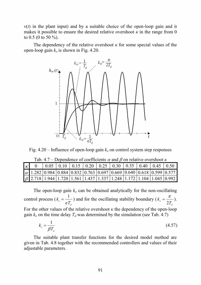
91
v(t) in the plant input) and by a suitable choice of the open-loop gain and it
makes it possible to ensure the desired relative overshoot κ in the range from 0
to 0.5 (0 to 50 %).
The dependency of the relative overshoot κ for some special values of the
open-loop gain ko is shown in Fig. 4.20.
Fig. 4.20 – Influence of open-loop gain ko on control system step responses
Tab. 4.7 – Dependence of coefficients and on relative overshoot κ
0 0.05 0.10 0.15 0.20 0.25 0.30 0.35 0.40 0.45 0.50
1.282 0.984 0.884 0.832 0.763 0.697 0.669 0.640 0.618 0.599 0.577
2.718 1.944 1.720 1.561 1.437 1.337 1.248 1.172 1.104 1.045 0.992
The open-loop gain ko can be obtained analytically for the non-oscillating
control process (d
oT
ke
1 ) and for the oscillating stability boundary (
d
oT
k2
).
For the other values of the relative overshoot κ the dependency of the open-loop
gain ko on the time delay Td was determined by the simulation (see Tab. 4.7)
d
oT
k
1 (4.57)
The suitable plant transfer functions for the desired model method are
given in Tab. 4.8 together with the recommended controllers and values of their
adjustable parameters.

92
The transfer function of the recommended controller GC(s) for some of the
plants with the transfer function GP(s) for the desired control transfer function
(4.56) can be obtained from the formula for direct synthesis
)(1
)(
)(
1)(
)()(1
)()()(
sG
sG
sGsG
sGsG
sGsGsG
wy
wy
P
C
PC
PCwy
(4.58)
Tab. 4.8 – Values of adjustable controller parameters for the desired model
method
Plant Controller <
analog T = 0
digital T > 0
Type
PK
IT DT
1 sTd
s
k e
1
P
1)(
1
kTT d – –
2 sTd
sT
k
e
11
1
PI
1)( kTT
T
d
I
21
TT
–
3
sTd
sTs
k
e
11
1
PD
1)(
1
kTT d –
21
TT
4 sTd
sTsT
k
e
11 21
1
21 TT
PID 1)( kTT
T
d
I
TTT 21
421
21 T
TT
TT
5
sTd
sTsT
k
e
12 00
22
0
1
15.0 0
PID 1)( kTT
T
d
I
TT 002 42 0
0 TT
E.g. for the plant with the transfer function
sT
P
d
sT
ksG
e
1)(
1
1
after substitution in (4.58) and considering (4.56) the controller transfer function
sT
ksk
sTk
ks
k
ks
k
k
sTsG
I
P
o
sT
sT
o
o
sT
sT
o
o
sTC
d
d
d
d
d *
*
1
1
1
11
1)1(
ee
1
ee
e
1)(
is obtained (see the row 2 in Tab. 4.8 for T = 0), where
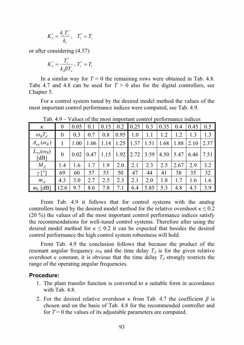
93
1
*
1
*
*, TT
k
TkK
I
Io
P
or after considering (4.57)
1
*
1
*
*, TT
Tk
TK
I
d
I
P
In a similar way for T = 0 the remaining rows were obtained in Tab. 4.8.
Tabs 4.7 and 4.8 can be used for T > 0 also for the digital controllers, see
Chapter 5.
For a control system tuned by the desired model method the values of the
most important control performance indices were computed, see Tab. 4.9.
Tab. 4.9 – Values of the most important control performance indices
κ 0 0.05 0.1 0.15 0.2 0.25 0.3 0.35 0.4 0.45 0.5
dRT 0 0.3 0.7 0.8 0.95 1.0 1.1 1.2 1.2 1.3 1.3
)( RwyA 1 1.00 1.06 1.14 1.25 1.37 1.51 1.68 1.88 2.10 2.37
Lwy(ωR)
[dB] 0 0.02 0.47 1.15 1.92 2.72 3.59 4.50 5.47 6.46 7.51
SM 1.4 1.6 1.7 1.9 2.0 2.1 2.3 2.5 2.67 2.9 3.2
γ [°] 69 60 57 53 50 47 44 41 38 35 32
Am 4.3 3.0 2.7 2.5 2.3 2.1 2.0 1.8 1.7 1.6 1.6
mL [dB] 12.6 9.7 8.6 7.8 7.1 6.4 5.85 5.3 4.8 4.3 3.9
From Tab. 4.9 it follows that for control systems with the analog
controllers tuned by the desired model method for the relative overshoot κ ≤ 0.2
(20 %) the values of all the most important control performance indices satisfy
the recommendations for well-tuned control systems. Therefore after using the
desired model method for κ ≤ 0.2 it can be expected that besides the desired
control performance the high control system robustness will hold.
From Tab. 4.9 the conclusion follows that because the product of the
resonant angular frequency ωR and the time delay Td is for the given relative
overshoot κ constant, it is obvious that the time delay Td strongly restricts the
range of the operating angular frequencies.
Procedure:
1. The plant transfer function is converted to a suitable form in accordance
with Tab. 4.8.
2. For the desired relative overshoot κ from Tab. 4.7 the coefficient β is
chosen and on the basis of Tab. 4.8 for the recommended controller and
for T = 0 the values of its adjustable parameters are computed.
94
SIMC method
The SIMC method comes from the internal model control (IMC). Its
author, Skogestad, recommends the abbreviation SIM to be understood as
„SIMple Control“ or „Skogestad IMC“.
For the determination of the controller transfer function the formula for
direct synthesis [see (4.58)]
)(1
)(
)(
1)(
sG
sG
sGsG
wy
wy
P
C
(4.59)
is used on the assumption that the control system transfer function has the form
sT
w
wyd
sTsG
e
1
1)( (4.60)
where Tw is the time constant of the closed-loop control system.
E.g. for the plant with the transfer function
sT
Pd
sT
ksG
e
1)(
1
1
it is obtained
sT
w
CdsTk
sTsG
e1
11)(
1
1 (4.61)
After use of the approximation
sTdsTd
1e
from relation (4.61) the transfer function of the PI controller
1
1
1 ,)(
,1
1)( TTTTk
TK
sTKsG I
dw
P
I
PC
is obtained.
By a suitable choice of the time constant Tw the different fast responses can
be obtained. The time constant Tw can be considered as the tuning parameter.
There is most often recommended Tw = Td and the integral time TI is determined
on the basis of the relation
)8,min( 1 dI TTT
Then the values of the adjustable parameters of the PI controller are given
(see rows 2 and 3 in Tab. 4.10)

95
ddI
dI
d
PTTTT
TTTT
Tk
TK
8for8
8for,
21
*
11
*
1
1*
In a similar way the remaining rows in Tab. 4.10 were obtained.
The cases in the rows 2, 4 and 6 in Tab. 4.10 are equivalent to the desired
model method for the relative overshoot κ ≈ 0.05 (5 %).
Tab. 4.10 – Values of adjustable controller parameters for the SIMC method
Plant Controller
Note Type
*
PK *
IT *DT
1 sTdk
e1 I – dTk12 – –
2 sTd
sT
k
e
11
1
PI
dTk
T
1
1
2 1T – dTT 81
3 dTk
T
1
1
2 dT8 – dTT 81
4
sTd
sTsT
k
e
)1)(1( 21
1
21 TT
PIDi dTk
T
1
1
2 1T 2T dTT 81
5 dTk
T
1
1
2 dT8 2T dTT 81
6
PID dTk
TT
1
21
2
21 TT
21
21
TT
TT
dTT 81
7 21
21
16
)8(
d
d
Tk
TTT
dTT 82
d
d
TT
TT
8
8
2
2
dTT 81
8 sTd
s
k e
1
PI
dTk12
1
dT8 – –
9 sTd
sTs
k
e
)1( 2
1
PIDi dTk12
1
dT8 2T –
10 PID 21
2
16
8
d
d
Tk
TT
dTT 82
d
d
TT
TT
8
8
2
2
–
11 sTd
s
k e
2
1
PIDi 2116
1
dTk dT8 dT8 –
12 PID 218
1
dTk dT16 dT4 –

96
Procedure:
1. The plant transfer function is converted to a suitable form in accordance
with Tab. 4.10.
2. For the recommended controller on the basis of Tab. 4.10 the values of
its adjustable parameters are computed.

97
5 DIGITAL CONTROL
This chapter is devoted to a brief description of the control systems with
digital controllers. A simple approximate design method for digital controllers is
shown.
Lately digital controllers have most frequently been used in control
engineering. It is caused by the recent development of digital technologies and
simultaneously the decreasing of their prices. Conventional digital controllers
mostly implement the same control algorithms, like analog ones but in discrete
forms. Further in the text it is supposed that the quantization error is
negligibly small and therefore the concept “digital” (discrete in magnitude and
time) and “discrete” (discrete in time but continuous in magnitude) are
equivalent. For example, the digital PID controller
D
D
I
k
iI
P
P
Dk
iI
P
TkekTeKiTeKkTeK
TkekTeT
TiTe
T
TkTeKkTu
])1[()()()(
])1[()()()()(
0
0
(5.1)
,2,1,0k
corresponds to the analog PID controller (3.19), where KP, KI and KD are the
proportional, summation and difference component weights, T – the
sampling period, kT – the discrete time.
From the adjustable digital PID controller parameters it holds that
T
TKK
T
TKK D
PD
I
PI , (5.2)
or
TK
KTT
K
KT
P
DD
I
PI , (5.3)
It is obvious that for the digital controllers the further adjustable parameter
arises – the sampling period T. Its proper choice is very important from the point
of view of control performance. The sampling period T increases the influence
of the summation component (the summation component always destabilizes the
control process) and decreases the influence of the difference component (the
difference component stabilizes the control process), therefore the sampling
period´s influence on the control performance and stability is always
negative. Also, from this follows that between the sampling instants
kT < t < (k + 1)T the digital controller hasn’t any information about the current

98
value of the control error e(t), see Fig. 5.1 and therefore it cannot perform and
control well.
Fig. 5.1 – Control error course in a control system with a digital controller
The analog-to-digital (A/D) converter processes the conversion from the
analog (continuous) variable to the digital (discrete) variable. It is often plugged
in the feedback (Fig. 5.2). The output variable of the digital controller (DC) is
the discrete control variable u(kT), which the digital-to-analog (D/A) converter
converts to the continuous in the time control variable uT(t) with a staircase
course (Fig. 5.3), which is the input variable of the plant (P).
Fig. 5.2 – Control system with a digital controller
Fig. 5.3 – Control variable courses in a control system with a digital controller
)(tu
2T 0 kT t
)(tuT
)(kTu
)(2
tuT
tu T
T4
T6 T8
T10
DC D/A P
A/D
)(kTw )(kTe )(kTu )(kTuT )(tv
)(ty
)(kTy
0 T T 2 T 3
T 4
kT
) ( kT e

99
From Fig. 5.3 it follows that the staircase control variable uT(t) for the
small sampling period T value can be substituted by smooth control variable
u(t), which is delayed by half the sampling period, i.e. u(t – T/2). It is obvious
that this substitution will be better for the smaller sampling period. Therefore for
the approximate analysis and synthesis of the control system with the digital
controller the substitute control system in Fig. 5.4 can be used. The digital
controller is substituted by the analog controller of the corresponding type and
the time delay is assigned to the plant. If methods not suitable for the time delay
are used for analysis or synthesis then the time delay must be approximated by
one of the following relations
sT
sT
sT
41
41
e 2
(5.4)
or
sT
sT
21
1e 2
(5.5)
The more accurate approximation is not used. The obtained results must be
carefully interpreted with a sense of the approximate approach.
Fig. 5.4 – Substitute control system with the digital controller
The digital PID controller is the most complex conventional controller. In
technical practice simpler digital controllers are used:
the digital PI controller
k
iI
PiTe
T
TkTeKkTu
0
)()()( (5.6)
the digital PD controller
])1[()()()( TkekTeT
TkTeKkTu D
P (5.7)
)(sW
)(sGC
)(sV
sT
2e
)(sGP
)(sY

100
the digital I controller
k
iI
iTeT
TkTu
0
)()( (5.8)
and the digital P controller
)()( kTeKkTu P (5.9)
The summation and difference components (terms) are often implemented
using other different methods (the forward rectangular method, trapezoidal
method etc.).
For the suitable choice of the sampling period T these distinctions aren’t
substantial and in addition the manufacturers very often don’t give any
information about the summation and difference component implementation.
For the digital difference component the input variable must be always
suitably filtered.
For choosing the sampling period T definite rules and recommendations
don´t exist. For a rough choice the following recommendations can be used.
Sampling period T Plant (Process)
(10 ÷ 500) μs the accurate control, the electrical and power
systems, the accurate control robots
(0.5 ÷ 20) ms the stabilization of the power systems, the flight
and drive simulators
(10 ÷ 100) ms image processing, virtual reality, artificial vision
(0.5 ÷ 1) s the control and monitoring of the processes, the
chemical processes, the power systems
(1 ÷ 3) s flow control
(1 ÷ 5) s pressure control
(5 ÷ 10) s level control
(10 ÷ 20) s temperature control
The more accurate determination of the sampling period comes from the
behavior of the plant or a closed-loop control system. For example, for the
proportional non-oscillating plant it is recommended that
95.06
1
15
1tT
(5.10)
where t0.95 is the time when the step response reaches 95 % of the steady-state
value.

101
For the plant with the dominant time delay Td the relation
dTT
3
1
8
1 (5.11)
is recommended.
For digital controllers with the difference component the sampling period T
must be chosen in accordance with the relation
DTT 5.01.0 (5.12)
Some controller tuning methods are processed and derived also for the
digital controllers (see Tab. 4.6 ÷ 4.8) and therefore they can be used directly.

102
6 TWO- AND THREE-POSITION CONTROL
The chapter is devoted to the two- and tree-position control, which belongs
among the simplest of control technologies.
The two- and three-position (relay) control is widely and commonly
used in home equipment and devices. Especially in every house, the two-
position (ON-OFF) control is used, e.g. for the electric iron temperature (see
Fig. 1.3), water temperature and the level in the washing machine, the room
temperature etc.
The main reason of the use of the two- and three-position control is its very
low price and relatively high reliability.
B B
B
B
B B
0 e
u
0 h
0 e
u
0 h
0 e
u
h
0 e
u
h
a) b)
Fig. 6.1 – Different characteristics of a two-position controller: a) asymmetric
without hysteresis (h = 0) and with hysteresis (h > 0), b) symmetric without
hysteresis (h = 0) and with hysteresis (h > 0)
2
a
2
a
B
2
a
2
a
B
BB
0 e
u
0h
0 e
u
h
h
Fig. 6.2 – Characteristic of a symmetric three-position controller without
hysteresis (h = 0) and with hysteresis (h > 0)

103
The two- and three-position controllers are strongly non-linear. Their
characteristics are relay characteristics shown in Figs 6.1 and 6.2, where B is the
relay amplitude, h – the hysteresis width, a – the dead zone. If the controller
characteristic is without hysteresis (i.e. without memory) then it is the controller
static characteristic. In the case of the controller characteristic with the
hysteresis (i.e. with memory) this characteristic isn’t in an exact sense “static”
and therefore it is just called the “characteristic”.
e
uw
2v
ye
1v
sTd
sT
k
e
11
1
Fig. 6.3 – Control system with ON-OFF controller
t
B
) ( t u
0
t
y Δ
y T
d T
d T d T
0
min y
d y
w
h y
1 T
1 T 1 T
B k y 1 max
) ( t y
0
h
B
e
u
ON
OFF
Fig. 6.4 – Courses of controlled y(t) and control u(t) variables in control system
with an ON-OFF controller
Two-position controllers with the characteristic as in Fig. 6.1a very often
operate in the mode “switch-on” and “switch-off” (e.g. the heating is on and the
heating is off) and as Fig. 6.1b they operate in the mode “switch-on plus” and

104
“switch-on minus” (e.g. the heating is on and the cooling is on). The three-
position controllers in Fig. 6.2 are the two-position controller (in Fig. 6.1b) with
extension of the third position “switch-off”. They often operate in mode
“switch-on plus”, “switch-off” and “switch-on minus” (e.g. the heating is on, the
heating and cooling are off and the cooling is on). The typical control system
with the ON-OFF controller is in Fig. 6.3. Since both the originals of the
variables and their transforms stand out the variables are written without their
arguments and in lower case letters. The operation of the control system in Fig.
6.3 is following. It is supposed that at the beginning the controlled variable
value is y(0) = ymin. Because e(0) > h/2 the control variable u(t) = B (the state:
switch – ON) and therefore the initial course of the controlled variable y(t) is
given by the relation (Fig. 6.4)
0),(e1)()( 1
minmaxmin
tTtyyyty d
T
Tt d
(6.1)
After reaching the value 2
)(h
wty the control variable u(t) = 0 (the
state: switch – OFF), the controlled variable y(t) at first rises during the time
delay Td and then it falls until it reaches the value 2
)(h
wty , the control
variable u(t) = B (the state: switch – ON), it further falls during the time delay Td
and then it rises etc. The whole control process periodically repeats. Because the
control system with the ON-OFF controller is strongly non-linear therefore the
analytical description of the course of the controlled variable y(t) is relatively
complicated. While its graphical construction is very easy and it follows directly
from Fig. 6.4.
For the well-designed control system with the ON-OFF controller the
desired variable (set-point) value approximately holds
2
minmax yyw
(6.2)
If it is equal then the 100 % abundance of the actuator power is given and
the average controlled variable value is yav = w. For the higher power abundance
the inequality yav > w holds and for the smaller one the opposite inequality yav <
w holds. In both the last cases the courses of the controlled variable y(t) are
asymmetric.
If the disturbance variables v1(t) and v2(t) influence the control system in
Fig. 6.3 they cause the controlled variable y(t) to fall under value 2
hw , the
control variable u(t) = B (the state: switch – ON), the controlled variable y(t)

105
after the time delay Td begins to rise and again the periodical control process
arises.
It is obvious that if the control error e(t) arises [it doesn’t matter whether it
was caused by the desired w(t) or disturbance v1(t) and v2(t) variables or by the
plant behavior change] then the ON-OFF controller makes efforts to remove it
by the maximum value of the control variable, i.e. umax = B or umin = 0.
Therefore if the ON-OFF control is applicable then it is highly robust.
The applicability of the ON-OFF control decides the obtained control
performance. It is given by the oscillation band width Δy of the controlled
variable, which can be determined on the basis of the relations (see Fig. 6.4)
11 e2
e122
maxmaxmax
T
T
T
T
h
dd
hwyy
hwy
hwy
11 e2
e122
minminmin
T
T
T
T
d
dd
yh
wyyh
wh
wy
11 ee1)(Δ minmax
T
T
T
T
dh
dd
hyyyyy
(6.3)
After using of the approximation
0and1e11
1
T
Th
T
T ddT
Td
the last relation in (6.3) can be simplified
hT
Tyyy d
1
minmax )(Δ (6.4)
From the approximate formula (6.4) it is obvious that both the hysteresis
width h and the time delay Td have a negative influence on the oscillation band
width Δy. The time delay Td can be sometimes decreased by the suitably placed
sensor but it is mostly given by the plant behavior and therefore it cannot be
decreased.
The time delay Td is the greatest enemy of the ON-OFF control (anywhere
in the control) and therefore it demands
2.0n
u
T
T (6.5)
would hold (in order to fulfil the condition Tu = Td = Td1, Tn = T1, see Fig. 3.6a).

106
Therefore if the desired control performance isn’t reached for h = 0, then
the ON-OFF controller cannot be used.
From a practical point of view the oscillating period Ty is very important
because its inverse value
y
yT
f1
(6.6)
expresses the switching frequency (i.e. number of switch-on or switch-off) per
time unit. The switching frequency fy has a direct influence on the lifetime of the
controller or actuator. From the Fig. 6.4, it follows that the oscillating period Ty
will be greater if the time delay Td and the hysteresis width h will be greater. It
is obvious that these requirements on the minimal oscillation band width Δy and
the maximal oscillation period Ty are contradictory to each other and therefore it
is necessary to choose a compromise solution.
For the electronic two-position controller the oscillation period Ty can be
increased by the adjustable dwell time.
It is obvious that all considerations can be applied to a two-position
symmetric controller (Fig. 6.1b) for ymin = – k1B.
The two-position symmetric controller (Fig. 6.1b) is sometimes used
together with the integrating device (most frequently with the electric drive). Its
disadvantage is the continuous switching, therefore the use of the three-position
controller (Fig. 6.2) is more suitable in accordance with Fig. 6.5. This
connection is often used for the actuator (valve) setting.
ue
s
k1
Fig. 6.5 – Three-position controller with integrating device
The great oscillating band width Δy for the two- and three-position
controllers can be decreased by the dynamic feedback, see Fig. 6.6. For both
interconnections in Fig. 6.6 the two- or three-position controller can be
approximately substituted by the gain kn → ∞ and then holds
)(1
1
)(1)(
)()(
sGk
sGk
k
sE
sUsG
FB
n
FBn
nC
)(
1)(
sGsGk
FB
Cn (6.7)
where GFB(s) is the feedback transfer function.

107
u e
) ( s G FB
) ( s G C
u e
) ( s G FB
) ( s G C
Fig. 6.6 – Two- and three-position controller with dynamic feedback
It is obvious that the two- or three-position controller with a dynamic
feedback approximately implements the inversion of the feedback, i.e. (6.7).
For example, for
1)(
sT
ksG
FB
FBFB
the approximate PD controller
FBD
FB
P
DP
FB
C
TTk
k
sTksGsE
sUsG
,1
)1()(
1
)(
)()(
(6.8)
can be obtained.
Similarly for
1)(
sT
sksG
FB
FBFB
the approximate PI controller
FBI
FB
FB
P
I
PC
TTk
Tk
sTk
sE
sUsG
,
)1
1()(
)()(
(6.9)
is obtained and for
21
21
,)1)(1(
)(FBFB
FBFB
FB
FBTT
sTsT
sksG

108
the approximate PIDi (with the interaction) controller is implemented [see
(3.24)]
21
1 ,,
)1)(1
1()(
)()(
FBDFBI
FB
FB
P
D
I
PC
TTTTk
Tk
sTsT
ksE
sUsG
(6.10)
The PI step controller is obtained for interconnection in accordance with
Fig. 6.7. Its transfer function is approximately given
FBIFB
FB
P
I
PC
TTTk
kk
sTk
sE
sUsG
,
)1
1()(
)()(
1
(6.11)
u e
1 s T
k
FB
FB
) ( s G C
s
k 1
Fig. 6.7 – PI step controller

109
7 CONCLUSION
After reading this book every control engineering student is now able to
understand what the control objective is, why negative feedback is important, when
open loop control can be used, and the four main principles for every general
system: the analysis, synthesis, identification and control.
In order to be able to see the behavior of systems when they respond to signals
on their inputs, the tools for modeling them and methods for visualizing the output
results are presented.
The analysis part starts with the role of controllers and their influence on the
stability of systems as well as methods on how to check them for that. The
synthesis part continues with a detailed look into controller tuning methods and
procedures, both for analog and digital control, so our reader can decide what is
more suitable, when, and under which conditions. A special chapter is devoted to
two- and three-position (relay) control, since it is widely and commonly used in
home equipment and devices.
For deeper study and a wider view, it is possible to use the recommended
references.

110
8 REFERENCES
ÅSTRÖM, K. – HÄGGLUND, T. Advanced PID Control. Instrument Society of
America, Research Triangle Park, 2006, 460 p.
CHEN, CH.T. Analog and Digital Control System Design: Transfer-Function,
State-Space, and Algebraic Methods. Oxford University Press, New York –
Oxford 1993, 600 p.
DORF, R.C. – BISHOP, R. Modern Control Systems (12th ed.). Prentice-Hall,
Upper Saddle River, New Jersey 2011, 1082 p.
FRANKLIN, G.F. – POWELL, J.D. – EMAMI-NAEINI, A. Feedback Control of
Dynamic Systems (4th ed.). Prentice-Hall, Upper Saddle River, New Jersey
2002, 910 p.
GÓRECKI, H., FUKSA, S., GRABOWSKI, P., KORYTOWSKI, A. Analysis and
Synthesis of Time Delay Systems. PWN-Polish Scientific Publishers – John
Wiley&Sons, Warszawa – Chichester, 1989, 369 p.
KOWAL, J. Podstawy automatyki (Tom I). Uczelniane wydawnictwa naukovo-
dydaktyczne AGH, Kraków, 2006, 301 str.
LANDAU, I.D. – ZITO, G. Digital Control Systems. Design, Identification and
Implementation. Springer-Verlag, London 2006, 484 p.
LEVINE, W.S. (Editor) The Control Handbook. CRC Press, Boca Raton, Florida
1996, 1548 p.
MIKLEŠ, J., FIKAR, M. Process Modelling, Identification, and Control. Springer-
Verlag, Berlin, 2007, 480 p.
NISE, N.S. Control Systems Engineering (2nd ed.). The Benjamin/Cummings
Publishing Company, Redwood City 1995, 851 p.
O’DWYER, A. Handbook of PI and PID Controllers Tuning Rules (3rd ed.).
Imperial College Press, World Scientific, London 2009, 608 p.
OGUNNAIKE, B.A. – RAY, W.H. Process Dynamics, Modeling and Control.
Oxford University Press, New York – Oxford 1994, 1260 p.
SKOGESTAD, S. Probably the Best Simple PID Tuning Rules in the World. Paper
No. 276h presented at AIChE Annual Meeting, pp. 1-28, Reno, USA,
November 19, 2001
SKOGESTAD, S. Simple Analytic Rules for Model Reduction and PID Controller
Tuning. Modeling, Identification and Control, Vol. 25, No. 2, 2004, pp. 52-
120
VÍTEČKOVÁ, M., VÍTEČEK, A. Základy automatické regulace. 2. Přepracované
vydání. FS VŠB-TUO, Ostrava, 2008, 244 str.

111
ZÍTEK, P. Time Delay Control System Design Using Functional State Models.
CTU Publishing House, Prague, 1998, 93 p.

112
1 LAPLACE TRANSFORM - BASIC RELATIONS AND PROPERTIES
Definition formulas
1
0
deL ttxtxsXst
2
jc
jc
stssX
jsXtx de
2
1L
1
Linearity
3 sXasXatxatxa 22112211L
Similarity theorem
4 0,L
a
a
sXatax
Convolution in time domain
5 sXsXsXsXdxtxdxtxtt
1221
0
12
0
21 LL
Real shifting in time domain (on the right)
6 0,eL
asXatxas
Real shifting in time domain (on the left)
7 0,deeL0
attxsXatx
astas
Complex shifting in complex domain
8 asXtxat
eL
Derivative in time domain
9 1 order derivative
0d
dL xssX
t
tx
10 n order derivative
n
ii
iinn
n
n
t
xssXs
t
tx
11
1
d
0d
d
dL
Derivative in complex variable domain
11 s
sXttx
d
dL
Integral in time domain
12 sXs
xt 1
dL0

113
Integral value
13 sXttxs 0
0
limd
14 s
sXtttx
s d
dlimd
00
Periodical function transform
15 as
sXatxatxtx
e1
12L a – period, a > 0
Initial value in time domain (if it exists)
16 ssXtxxst
limlim00
Final value in time domain (if it exists)
17 ssXtxxst 0limlim
Mathematical operation with respect to independent parameter
18 asXatx ,,L
19 asXatxaaaa
,lim},limL{00
20
a
asX
a
atx
,,L
21
2
1
2
1
d,d,La
a
a
a
aasXaatx
Inverse transform by residues
22
i
strir
r
ssi
st
i sssXss
srsXtx
i
i
i
ii
ed
dlim
!1
1eres
1
1
ri – the multiplicity of transform pole si
i
irn
– the polynomial degree in the transform denominator

114
2 LAPLACE TRANSFORM - CORRESPONDENCES
Transform X(s) Original x(t)
1 s t
2 1 t
3 s
1
t
4 ,2,1,1
nsn
!1
1
n
tn
5 11 sT
s ,e 1
11t
t
1
1
1
T
6 1
1
1 sT ,e 1
1t
1
1
1
T
7 1
1
1 sTs
,e1 1t
1
1
1
T
8 1
1
12
sTs
,1e1
1
1
tt
1
1
1
T
9 1
1
1
1
sTs
sb ,e11 1
11t
b
1
1
1
T
10 1
1
12
1
sTs
sb
,1
,e11
1111
bCtC
t 1
1
1
T
11 21 1sT
s
,e1 1
121
tt
1
1
1
T
12 21 1
1
sT
,e 121
tt
1
1
1
T
13 2
1 1
1
sTs
,e11 1
1t
t
1
1
1
T
14 21
21
1
sTs
,e22
1
11
ttt
1
1
1
T
15 21
1
1
1
sT
sb
,e1 1
11121
ttbb
1
1
1
T
16 2
1
1
1
1
sTs
sb
,e111 1
111t
tb
1
1
1
T

115
Transform X(s) Original x(t)
17 21
2
1
1
1
sTs
sb
1
1112
1
11
211
1,1,
2
e 1
TbCbC
tCCCtt
18
,3,2,11
nsT
sn
,e1!1
1
1
2
1t
nn
tnn
t
1
1
1
T
19
,2,1,1
1
1
nsT
n
,e!1
1
1
1t
nn
n
t
1
1
1
T
20
,2,1,1
1
1
nsTs
n
,!
e11
0
11
n
i
iit
i
t
1
1
1
T
21
,2,1,1
1
12
nsTs
n
,!
e1
0
11
1
1
n
i
iit
i
tin
nt
1
1
1
T
22
21
21
,11
TTsTsT
s
122
2
121
1
2
2
1
121
1,
1
1,
1,ee 21
TTTC
TTTC
TTCC
tt
23
21
21
,11
1TT
sTsT
2
2
1
1
21
11
1,
1,
1,ee 21
TTTTCC
tt
24
21
21
,11
1TT
sTsTs
12
22
12
11
2
2
1
121
,
1,
1,ee1 21
TT
TC
TT
TC
TTCC
tt
25
21
212
,11
1TT
sTsTs
2
2
1
1
21
22
2
21
21
1
210210
1,
1,,
,ee 21
TTTT
TC
TT
TC
TTCCCCttt
26
21
21
1,
11
1TT
sTsT
sb
212
122
211
111
2
2
1
121
,
1,
1,ee 21
TTT
bTC
TTT
bTC
TTCC
tt
27
21
21
1,
11
1TT
sTsTs
sb
21
122
21
111
2
2
1
121
,
1,
1,ee1 21
TT
bTC
TT
TbC
TTCC
tt

116
Transform X(s) Original x(t)
28
21
212
1,
11
1TT
sTsTs
sb
2
2
1
1
12
2122
12
1111
1210210
1,
1,,
,ee 21
TTTT
TbTC
TT
TTbC
bTTCCCCttt
29 different
,3,2,
11
i
n
ii
T
n
sT
s
i
in
ikk
ki
ni
i
n
i
ti
TTT
TCC i
1,,e
,1
3
1
30 different
,3,2,
1
1
1
i
n
ii
T
n
sT
i
in
ikk
ki
ni
i
n
i
ti
TTT
TCC i
1,,e
,1
2
1
31 different
,3,2,
1
1
1
i
n
ii
T
n
sTs
i
in
ikk
ki
ni
i
n
i
ti
TTT
TCC i
1,,e1
,1
1
1
32 different
,3,2,
1
1
1
2
i
n
ii
T
n
sTs
i
i
n
i
ti
TCCt i
1,e
1
0
n
i
in
ikk
ki
ni
i TC
TT
TC
1
0
,1
,
33 22
s tsin
34 22 s
s tcos
35
10
,12
0
0022
0
sTsT
s
arctg,11
,1
,sine
20
0
0
0
30
11
T
TTCtC
t
36
10
,12
1
0
0022
0
sTsT
20
00
0
20
11 11
,,1
,sine
TTTCtC
t
37 10
,12
1
0
0022
0
sTsTs
arctg,11
,1
,sine1
20
0
0
0
0
11
T
TTCtC
t
38 10
,12
1
0
0022
02
sTsTs
arctg,11
,,1
2,2sine
20
00
01
200010
TTC
TCtCCtt

117
Transform X(s) Original x(t)
39
10
,12
1
0
0022
0
1
sTsT
sb
1
120
00
0
21
2013
0
11
1arctg,1
1,
211
,sine
b
b
TT
bTbT
CtCt
40 10
,12
1
0
0022
0
1
sTsTs
sb
201
202
0
00
0
21
2012
0
11
arctg,11
,
211
,sine1
Tb
T
TT
bTbT
CtCt
b1, b2 – the real constants, Ti > 0, i = 0, 1,...
118
Authors:
Prof. Ing. Antonín Víteček, CSc., Dr.h.c.
Prof. Ing. Miluše Vítečková, CSc.
Doc. Ing. Lenka Landryová, CSc.
Department: Control Systems and Instrumentation
Title: Basic Principles of Automatic Control
Place, Year, Edition: Ostrava, 2012, 1st
Pages: 118
Published:
VŠB – Technical University of Ostrava
17. listopadu 15/2172
708 33 Ostrava - Poruba
ISBN 978-80-248-4062-8


![Principles of solar control [Kompatibilit tsmodus]icebauhaus.sudile.com › images › 6 › ...of_solar_control.pdf · Principles of Solar Control, 19.06.2012 Helmut F.O. Müller,](https://static.dokumenty.site/doc/80x56/5ed3bffba0e09216242fe250/principles-of-solar-control-kompatibilit-tsmodus-a-images-a-6-a-ofsolarcontrolpdf.jpg)


