61
Brno University of Technology
Università degli Studi dell'Aquila
Mathematical Engineering
Laurea Specialistica in Ingegneria Matematica
Numerical study of the fluid motion and
mixing processes in the vitreous cavity
Author: Karel Pavl·
Supervisor: Rodolfo Repetto
Referee: Libor ermák
2007/2008

Abstract
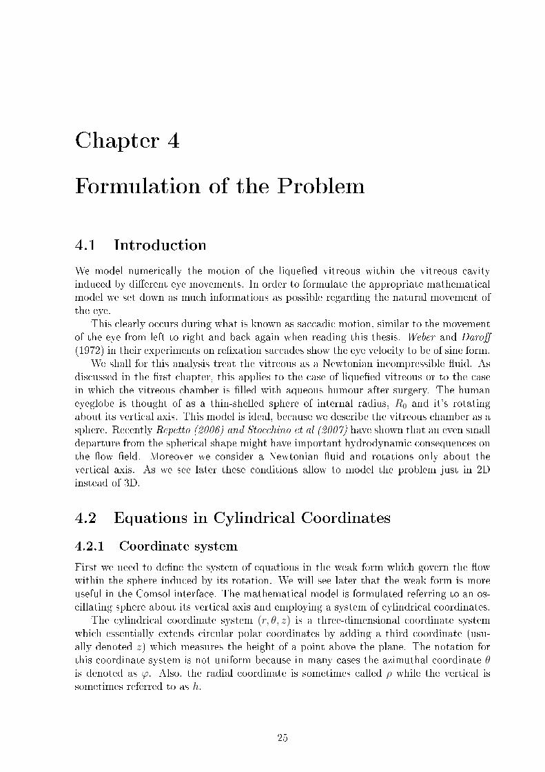
The vitreous cavity, the largest chamber of the eye, is delimited anteriorly by the lens andposteriorly by the retina and is lled by the vitreous humour. Under normal conditionsthe vitreous humour has the consistency of a gel, however, typically, with advancing agea disintegration of the gel structure occurs, leading to a vitreous liquefaction. Moreover,after a surgical procedure called vitrectomy the vitreous body may be completely removedand replaced by tamponade uids.
Besides allowing the establishment of an unhindered path of light from the lens tothe retina, the vitreous also has important mechanical functions. In particular, it has therole of supporting the retina in contact to the outer layers of the eye, and of acting as adiusion barrier for molecule transport between the anterior and the posterior segmentsof the eye.
Studying the dynamics of the vitreous induced by eye rotations (saccadic movements)is important in connection of both the above aspects. On the one hand indications existthat the shear stress exerted by the vitreous on the retina may be connected with theoccurrence of retinal detachment. On the other hand, if the vitreous motion is intenseenough (a situation occurring either when the vitreous is liqueed or when it has beenreplaced with a uid after vitrectomy), advective transport may be by far more importantthan diusion and may have complex characteristics. Advection has indeed been shownto play an important role in the transport phenomena within the vitreous cavity, but, sofar, only advection due to the slow overall uid ux from the anterior to the posteriorsegments of the eye has been accounted for, while uid motion due to eye rotations, evenif it is generally believed to play an important role, has been invariably disregarded.
Some recent contributions have pointed out the importance of accounting for the realvitreous cavity shape in studying uid motion induced by eye rotations. Modelling thevitreous cavity as a deformed sphere, showed that the ow eld displays very complexthree- dimensional characteristics to which eective uid mixing is likely to be associated.
The purpose of the thesis is to model numerically the motion of the liqueed vitreouswithin the vitreous cavity induced by dierent eye movements. Create the model in theComsol interface, compare the results with theoretical, experimental measurements anddo some ow visualizations. Finally show the dependence of the streaming intensity fromthe amplitude of rotations ε and the Womersley number α.
Key words
Comsol, uid motion, vitreous cavity, saccadic movements, retinal detachment.

PAVL, K. : Numerical study of the uid motion and mixing processes in the vitreouscavity, L`Aquila, The University of L`Aquila, Faculty of Engineering, 2008 (54 pages),Supervisor Rodolfo Repetto, Referee Libor ermák.
Statement
This is to certify that I wrote this thesis Numerical study of the uid motion and mixingprocesses in the vitreous cavity on my own and that the references include all the sourcesof information I have utilized.
L`Aquila June 26, 2008 Karel Pavl·
Acknowledgement
I would like to express my gratitude to Rodolfo Repetto who provided me with a chal-lenging and interesting topic for my diploma thesis. Rodolfo`s constant support, hisencouragement and continuous guidance have greatly contributed to the success of thiswork and are highly appreciated. Thanks a lot!I also want to take the time to thank all those who have aided me in the creation of thisthesis work. In alphabetical order, these are Alessandro Testa, prof. Amabile Tatone andElisa Colangeli.I am also indebted to everyone who has supported my studies at the University of L`Aquilanamely prof. Josef Slapal, prof. Bruno Rubino and Danilo Larivera. Thanks a lot, it wasa great experience for me to study in Italy for the last academic year.Last but not least, I want to thank all my family and friends who have supported meduring my studies and thus had an important share in the successful completion of thisthesis. In random order, these would be my mother, my sister, my girlfriend Marketaand the whole crazy bunch of friends out there, you know who you are. Thank you verymuch, your help is greatly appreciated.
Karel Pavl·

Contents
1 Introduction 3
1.1 The Human Eye . . . . . . . . . . . . . . . . . . . . . . . . . . . . . . . . . 31.1.1 Anatomy . . . . . . . . . . . . . . . . . . . . . . . . . . . . . . . . . 31.1.2 Defects of the Eye . . . . . . . . . . . . . . . . . . . . . . . . . . . 41.1.3 Vitreous Body, PVD and RD . . . . . . . . . . . . . . . . . . . . . 51.1.4 Fluid Motion . . . . . . . . . . . . . . . . . . . . . . . . . . . . . . 71.1.5 Saccadic movements . . . . . . . . . . . . . . . . . . . . . . . . . . 8
2 Experiments and Theory 9
2.1 PIV . . . . . . . . . . . . . . . . . . . . . . . . . . . . . . . . . . . . . . . 92.1.1 Previous Experiments . . . . . . . . . . . . . . . . . . . . . . . . . 92.1.2 Experimental Set-up . . . . . . . . . . . . . . . . . . . . . . . . . . 102.1.3 Steady Streaming . . . . . . . . . . . . . . . . . . . . . . . . . . . . 11
2.2 Theoretical Work . . . . . . . . . . . . . . . . . . . . . . . . . . . . . . . . 12
3 Finite Element Method, Comsol 17
3.1 FEM . . . . . . . . . . . . . . . . . . . . . . . . . . . . . . . . . . . . . . . 173.1.1 An Introduction to the Finite Element Method . . . . . . . . . . . 17
3.2 Mathematical Models . . . . . . . . . . . . . . . . . . . . . . . . . . . . . . 183.3 Numerical Simulations . . . . . . . . . . . . . . . . . . . . . . . . . . . . . 183.4 The Finite Element Method . . . . . . . . . . . . . . . . . . . . . . . . . . 18
3.4.1 The Basic Idea . . . . . . . . . . . . . . . . . . . . . . . . . . . . . 183.4.2 The Basic Features . . . . . . . . . . . . . . . . . . . . . . . . . . . 193.4.3 Simple Example . . . . . . . . . . . . . . . . . . . . . . . . . . . . . 203.4.4 Some Remarks . . . . . . . . . . . . . . . . . . . . . . . . . . . . . 233.4.5 Summary . . . . . . . . . . . . . . . . . . . . . . . . . . . . . . . . 23
3.5 What is COMSOL . . . . . . . . . . . . . . . . . . . . . . . . . . . . . . . 24
4 Formulation of the Problem 25
4.1 Introduction . . . . . . . . . . . . . . . . . . . . . . . . . . . . . . . . . . . 254.2 Equations in Cylindrical Coordinates . . . . . . . . . . . . . . . . . . . . . 25
4.2.1 Coordinate system . . . . . . . . . . . . . . . . . . . . . . . . . . . 254.2.2 Weak Form of the Equations . . . . . . . . . . . . . . . . . . . . . . 274.2.3 Derivation of the Weak Form of the Equations . . . . . . . . . . . . 284.2.4 Boundary and Incompressibility Conditions . . . . . . . . . . . . . 304.2.5 Dimensionless Form of the Governing Equation . . . . . . . . . . . 304.2.6 Scaling Boundary and Incompressibility Conditions . . . . . . . . . 33
1
5 Numerical Runs 34
5.1 Comsol Setup . . . . . . . . . . . . . . . . . . . . . . . . . . . . . . . . . . 345.1.1 Problem Denition . . . . . . . . . . . . . . . . . . . . . . . . . . . 345.1.2 Main Settings . . . . . . . . . . . . . . . . . . . . . . . . . . . . . . 345.1.3 Some Remarks . . . . . . . . . . . . . . . . . . . . . . . . . . . . . 37
6 Results-Comparisons 38
6.1 Steady Streaming . . . . . . . . . . . . . . . . . . . . . . . . . . . . . . . . 386.1.1 Extraction of the Steady Streaming . . . . . . . . . . . . . . . . . . 396.1.2 Streaming Intensity versus the Amplitude of Rotations . . . . . . . 436.1.3 Streaming Intensity for dierent values of the Womersley number . 44
7 Conclusions 45
8 Appendix 47
8.1 Plots . . . . . . . . . . . . . . . . . . . . . . . . . . . . . . . . . . . . . . . 47
2
Chapter 1
Introduction
1.1 The Human Eye
1.1.1 Anatomy
The human eye is the organ which gives us the sense of sight, allowing us to learn moreabout the surrounding world than we do with any of the other four senses. We use oureyes in almost every activity we perform, whether reading, working, watching television,writing a letter, driving a car, and in countless other ways. I think that most peopleprobably would agree that sight is the sense they value more than all the rest. The eyeallows us to see and interpret the shapes, colors, and dimensions of objects in the worldby processing the light they reect or emit. The eye is able to detect bright light or dimlight, but it cannot sense objects when light is absent.
Process of vision - light waves from an object enter the eye rst through the cornea,the clear dome at the front of the eye. The light then progresses through the pupil, thecircular opening in the center of the colored iris. Fluctuations in incoming light changethe size of the eye's pupil. For example when the light entering the eye is bright enough,the pupil will get smaller. Initially, the light waves are bent rst by the cornea, and thenfurther by the crystalline lens (located behind the iris and the pupil), to a nodal point(N) located immediately behind the back surface of the lens. At that point, the imagebecomes reversed (turned backwards) and inverted (turned upside-down). The light con-tinues through the vitreous humor, the clear gel, and then, ideally, back to a clear focus onthe retina, behind the vitreous. The small central area of the retina is the macula, whichprovides the best vision of any location in the retina. Within the layers of the retina, lightimpulses are changed into electrical signals which are sent through the optic nerve, alongthe visual pathway, to the occipital cortex at the posterior (back) of the brain. Here, theelectrical signals are interpreted by the brain as a visual image. So we can say that, wedo not "see" with our eyes but, rather, with our brains. Basically, eyes are the beginningsof the visual process.
Structure - the average newborn's eyeball is about 18 millimeters in diameter, fromfront to back (axial length). In an infant, the eye grows slightly to a length of approxi-mately 19 mm. The eye continues to grow, gradually, to a length of about 24-25 mm inadulthood. The eyeball is set in a protective cone-shaped cavity in the skull called theorbit. This bony orbit also enlarges as the eye grows, and is surrounded by layers of soft,fatty tissue. These layers protect the eye and enable it to turn easily. Traversing the
3
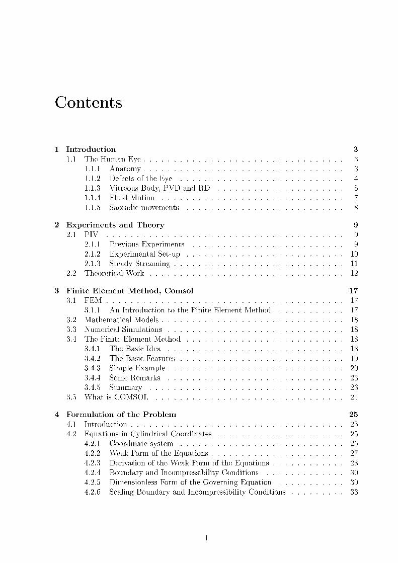
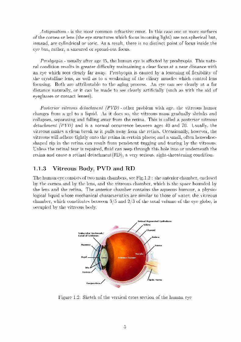
fatty tissue are three pairs of extraocular muscles, which regulate the motion of each eye.Several structures compose the human eye, the most important anatomical componentsare the cornea, conjunctiva, iris, crystalline lens, vitreous humor, retina, macula, opticnerve, and extraocular muscles, see Fig.1.1.
Figure 1.1: Anatomy of the eye - 1)Posterior chamber 2)Ora serrata 3)Ciliary mus-cle 4)Ciliary zonules 5)Canal of Schlemm 6)Pupil 7)Anterior chamber 8)Cornea 9)Iris10)Lens cortex 11)Lens nucleus 12)Ciliary process 13)Conjunctiva 14)Inferior obliquemuscle 15)Inferior rectus muscle 16)Medial rectus muscle 17)Retinal arteries and veins18)Optic disc 19)Dura mater 20)Central retinal artery 21)Central retinal vein 22)Opti-cal nerve 23)Vorticose vein 24)Bulbar sheath 25)Macula 26)Fovea 27)Sclera 28)Choroid29)Superior rectus muscle 30)Retina
1.1.2 Defects of the Eye
As we know the eye is not a perfect organ of the human body. The eye itself has manydefects as of all the other parts of the body. Some of these defects are listed below :
Myopia, Hyperopia - if the incoming light from a far away object focuses before it getsto the back of the eye, that eye's refractive error is called myopia (nearsightedness). Ifincoming light has not focused by the time it reaches the back of the eye, that eye's re-fractive error is hyperopia (farsightedness).
4
Astigmatism - is the most common refractive error. In this case one or more surfacesof the cornea or lens (the eye structures which focus incoming light) are not spherical but,instead, are cylindrical or toric. As a result, there is no distinct point of focus inside theeye but, rather, a smeared or spread-out focus.
Presbyopia - usually after age 45, the human eye is aected by presbyopia. This natu-ral condition results in greater diculty maintaining a clear focus at a near distance withan eye which sees clearly far away. Presbyopia is caused by a lessening of exibility ofthe crystalline lens, as well as to a weakening of the ciliary muscles which control lensfocusing. Both are attributable to the aging process. An eye can see clearly at a fardistance naturally, or it can be made to see clearly articially (such as with the aid ofeyeglasses or contact lenses).
Posterior vitreous detachment (PVD) - other problem with age, the vitreous humorchanges from a gel to a liquid. As it does so, the vitreous mass gradually shrinks andcollapses, separating and falling away from the retina. This is called a posterior vitreousdetachment (PVD) and is a normal occurrence between ages 40 and 70. Usually, thevitreous makes a clean break as it pulls away from the retina. Occasionally, however, thevitreous will adhere tightly onto the retina in certain places; and a small, often horseshoe-shaped rip in the retina can result from persistent tugging and tearing by the vitreous.Unless the retinal tear is repaired, uid can seep through this hole into or underneath theretina and cause a retinal detachment(RD), a very serious, sight-threatening condition.
1.1.3 Vitreous Body, PVD and RD
The human eye consists of two main chambers, see Fig.1.2 : the anterior chamber, enclosedby the cornea and by the lens, and the vitreous chamber, which is the space bounded bythe lens and the retina. The anterior chamber contains the aqueous humour, a physio-logical liquid whose mechanical characteristics are similar to those of water; the vitreouschamber, which constitutes between 3/5 and 2/3 of the total volume of the eye globe, isoccupied by the vitreous body.
Figure 1.2: Sketch of the vertical cross section of the human eye
5
The vitreous is a clear, gel-like material and has the following composition:
1. water (99%),2. a network of collagen brils,3. large molecules of hyaluronic acid,4. peripheral cells (hyalocytes),5. inorganic salts,6. sugar, and7. ascorbic acid.
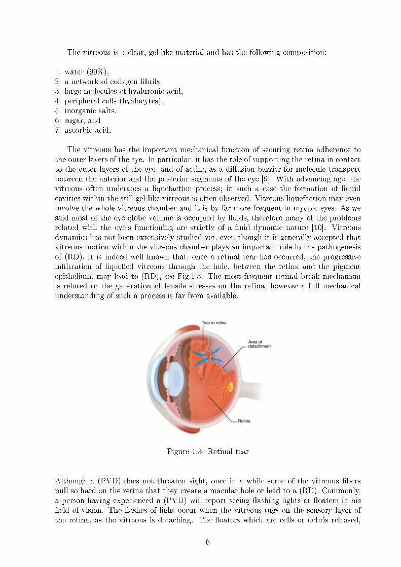
The vitreous has the important mechanical function of securing retina adherence tothe outer layers of the eye. In particular, it has the role of supporting the retina in contactto the outer layers of the eye, and of acting as a diusion barrier for molecule transportbetween the anterior and the posterior segments of the eye [9]. With advancing age, thevitreous often undergoes a liquefaction process; in such a case the formation of liquidcavities within the still gel-like vitreous is often observed. Vitreous liquefaction may eveninvolve the whole vitreous chamber and it is by far more frequent in myopic eyes. As wesaid most of the eye globe volume is occupied by uids, therefore many of the problemsrelated with the eye's functioning are strictly of a uid dynamic nature [10]. Vitreousdynamics has not been extensively studied yet, even though it is generally accepted thatvitreous motion within the vitreous chamber plays an important role in the pathogenesisof (RD). It is indeed well known that, once a retinal tear has occurred, the progressiveinltration of liqueed vitreous through the hole, between the retina and the pigmentepithelium, may lead to (RD), see Fig.1.3. The most frequent retinal break mechanismis related to the generation of tensile stresses on the retina, however a full mechanicalunderstanding of such a process is far from available.
Figure 1.3: Retinal tear
Although a (PVD) does not threaten sight, once in a while some of the vitreous berspull so hard on the retina that they create a macular hole or lead to a (RD). Commonly,a person having experienced a (PVD) will report seeing ashing lights or oaters in hiseld of vision. The ashes of light occur when the vitreous tugs on the sensory layer ofthe retina, as the vitreous is detaching. The oaters which are cells or debris released,
6
when the vitreous detaches can appear as little dots, circles, lines, cobwebs, or clouds.Floaters can be apparent especially when looking at a bright background, as the lightentering the eye casts shadows of the oaters onto the retina. The percent chance ofhaving a vitreous detachment is at least the same as one's age. As a (PVD) occurs thatis, as the vitreous uid separates from the retina organic debris or particles known as"oaters"(ying ies) are released. Most oaters are merely compressed cells or strandsof the vitreous gel which have clumped together so that they are less transparent thanthe rest of the vitreous. Some oaters are remnants of the hyaloid artery, which usuallydisintegrates before birth. These types of oaters are harmless. Floaters sometimes in-terfere with vision, often during reading, and they can be quite annoying. If a oaterappears directly in the line of sight, the best thing to do is to move the eye from side toside or up and down. Doing so can create a current within the internal uids to move theoater temporarily away from the line of sight. If a oater is suspended in a portion ofvitreous humor which is very viscous, it can be particularly persistent and bothersome.Unfortunately, in most instances, there is nothing to do but learn to tolerate the oaterspresence. Doctors in an extreme cases do surgical removal, called vitrectomy when thevitreous body may be completely removed and replaced by tamponade uids.
Studying the dynamics of the vitreous induced by eye rotations is important in con-nection of the above aspects. On the one hand indications exist that the shear stressexerted by the vitreous on the retina may be connected with the occurrence of retinaldetachment [10]. On the other hand, if the vitreous motion is intense enough (a situationoccurring either when the vitreous is liqueed or when it has been replaced with a uidafter vitrectomy), advective transport may be by far more important than diusion andmay have complex characteristics. Advection has indeed been shown to play an importantrole in the transport phenomena within the vitreous cavity, but, so far, only advectiondue to the slow overall uid ux from the anterior to the posterior segments of the eye hasbeen accounted for [2][7], while uid motion due to eye rotations, even if it is generallybelieved to play an important role [7], has been invariably disregarded.
1.1.4 Fluid Motion
Clearly the uid motion in the eye provides a possible mechanism for increasing detach-ment of the retina from the retinal pigment epithelium once a tear has occurred. Retinaldetachment, which may occur due to increased wall shear stress in a post-vitrectomy eye,caused by the uid ows. There are two main mechanisms for these ows.
1) The front of the eye is exposed to the cold atmosphere, means that the frontwall of the posterior chamber is a slightly lower temperature than the back wall. Thecooler uid will have a slightly higher density, so it tends to sink, which in turn drives aow throughout the posterior chamber.
2)The eyeball will move due to head motion, and also due to rotations of the eye-ball within its orbit (both voluntary and involuntary). These motions drive a ow in theposterior chamber.
Dyson et al (2004) show on the basis of simple calculations that motion due to eyerotations is expected to be by far more important that temperature-driven motion. In
7
present work we proceed to investigate the nature of ows driven only by the second ofthese mechanisms by constructing a model for the eyeball-motion-driven ow, and wespecialize to a model of saccadic motion of the eye.
1.1.5 Saccadic movements
Eyes are subject to various kinds of movements [11]. Our eyes are still continuously mov-ing, making two to three 'saccades' per second. When we scan a visual scene with quickeye movements known as saccades, the retina sends a series of 'snapshot' images to thebrain that must be integrated properly. Saccadic eye movements, due to their character-istics, are the most important in inducing vitreous motion within the vitreous chamber.Saccadic motion of the eye, i.e. rapid movement of the head or eyeball, will cause uidow in the posterior section of the eye. Saccadic motion occurs many times every day fora number of reasons. Some of them are : turning one's head or eyes to look at an objectof interest perceived in the peripheral vision; during reading; small amplitude intrusionswhilst xating on an object. Other possible eye movements are : the rapid eye movement(REM) that occurs during approximately four periods in a night's sleep; slow eye move-ment (SEM) during sleep onset; less frequently, there may also be more violent causes,such as being struck on the head.
It is clear that the saccadic motion has the potential to cause ow in the posteriorsegment of the eye. Some basic features of saccadic eye movements are as follows :
1) a very high initial angular acceleration (up to 30 000s−2 );
2) a somewhat less intense deceleration that is nevertheless capable of inducing avery ecient stop of the movement;
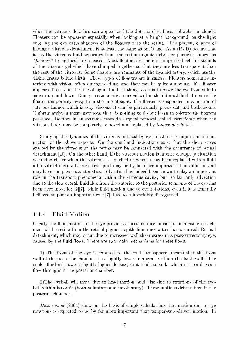
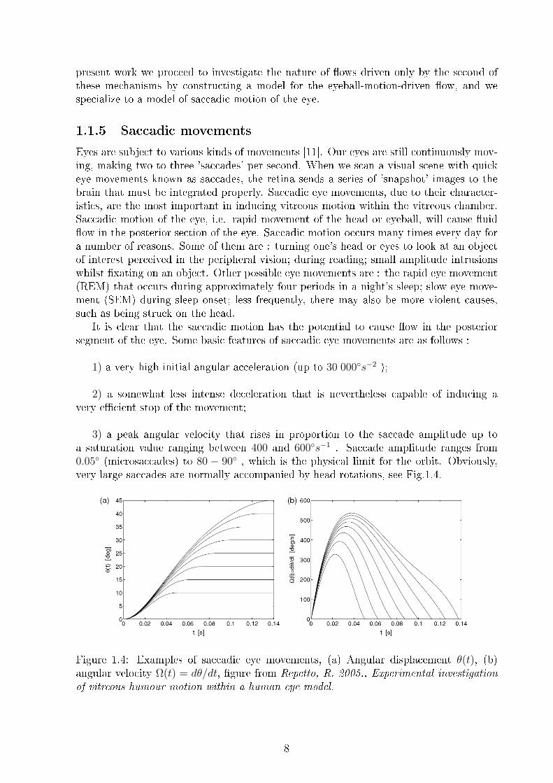
3) a peak angular velocity that rises in proportion to the saccade amplitude up toa saturation value ranging between 400 and 600s−1 . Saccade amplitude ranges from0.05 (microsaccades) to 80 − 90 , which is the physical limit for the orbit. Obviously,very large saccades are normally accompanied by head rotations, see Fig.1.4.
Figure 1.4: Examples of saccadic eye movements, (a) Angular displacement θ(t), (b)angular velocity Ω(t) = dθ/dt, gure from Repetto, R. 2005., Experimental investigationof vitreous humour motion within a human eye model.
8
Chapter 2
Experiments and Theory
2.1 PIV
2.1.1 Previous Experiments
The vitreous humour is the substance lling the vitreous chamber of the human eye. Leeet al. (1992) have studied the rheology of vitreous, showing that, in normal conditions, itbehaves as a viscoelastic material. Usually, with advancing age the vitreous undergoes aliquefaction process. In 1933 Lindner performed some experiments aimed at understand-ing the structure of the ow eld induced by eye rotations within the vitreous chamber.Later in 1976 Rosengren and Ostrelin reconsidered the previous experiments and pointedout the importance of eye rotations on the dynamics of vitreous. They just got a qual-itative picture of the hydrodynamic events within the eye. The model of the eye was acylinder which is strange because we know sphere represents better the real shape of thevitreous chamber. However, all these experiments did not take account into the scaleeects which arises from dierence in size between the model and the eye.
The main research was done by David et al. (1998). He showed that the uid motionin the inner part of the domain is out of phase with respect to the wall motion. He alsoshowed that the wall shear stress increases with the sphere radius giving a possible expla-nation of the more frequent occurrence of retinal detachments in myopic eyes, typicallycharacterized by a larger size. David et al. (1998) showed that the elastic component ofthe vitreous behaviour plays a fairly minor role with respect to the viscous one and thatthere is no dependence between the maximum shear stress at the wall and the elastic com-ponent of the vitreous behaviour. The shear stress is one of the most important quantityto be known in order to understand connection between vitreous motion and (RD).
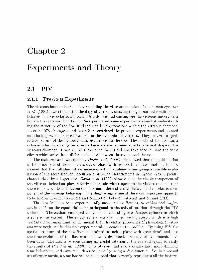
The ow eld has been experimentally measured by Repetto, Stocchino and Caer-ata in 2005, on the equatorial plane orthogonal to the axis of rotation, through the PIVtechnique. The authors employed an eye model consisting of a Perspex cylinder in whicha sphere was carved. The empty sphere was then lled with glycerol, which is a highviscosity Newtonian uid; which means that the elastic properties of physiological vitre-ous were neglected in this rst experimental approach to the problem. By using PIV thespatial structure of the ow eld is obtained in such a plane with great detail and alsothe time evolution of the ow can be suitably described. Two sets of experiments havebeen done. The rst is by considering sinusoidal rotation of the eye and trying to verifythe results of David et al. (1998). It is obvious that real saccades have more dierenttime behaviour, and cannot be described just by using a sine function. So, in a secondset of experiments, a time law has been adopted that correctly reproduces all the features
9
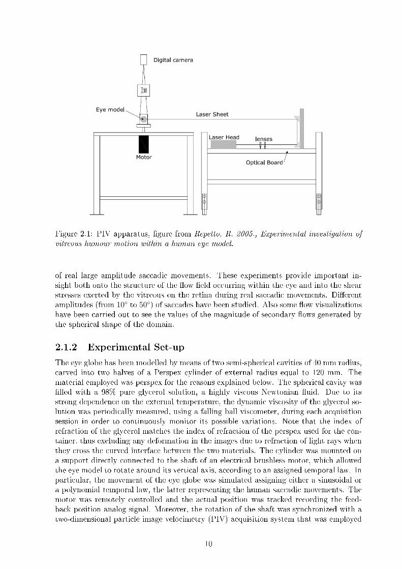
Figure 2.1: PIV apparatus, gure from Repetto, R. 2005., Experimental investigation ofvitreous humour motion within a human eye model.
of real large amplitude saccadic movements. These experiments provide important in-sight both onto the structure of the ow eld occurring within the eye and into the shearstresses exerted by the vitreous on the retina during real saccadic movements. Dierentamplitudes (from 10 to 50) of saccades have been studied. Also some ow visualizationshave been carried out to see the values of the magnitude of secondary ows generated bythe spherical shape of the domain.
2.1.2 Experimental Set-up
The eye globe has been modelled by means of two semi-spherical cavities of 40 mm radius,carved into two halves of a Perspex cylinder of external radius equal to 120 mm. Thematerial employed was perspex for the reasons explained below. The spherical cavity waslled with a 98% pure glycerol solution, a highly viscous Newtonian uid. Due to itsstrong dependence on the external temperature, the dynamic viscosity of the glycerol so-lution was periodically measured, using a falling ball viscometer, during each acquisitionsession in order to continuously monitor its possible variations. Note that the index ofrefraction of the glycerol matches the index of refraction of the perspex used for the con-tainer, thus excluding any deformation in the images due to refraction of light rays whenthey cross the curved interface between the two materials. The cylinder was mounted ona support directly connected to the shaft of an electrical brushless motor, which allowedthe eye model to rotate around its vertical axis, according to an assigned temporal law. Inparticular, the movement of the eye globe was simulated assigning either a sinusoidal ora polynomial temporal law, the latter representing the human saccadic movements. Themotor was remotely controlled and the actual position was tracked recording the feed-back position analog signal. Moreover, the rotation of the shaft was synchronized with atwo-dimensional particle image velocimetry (PIV) acquisition system that was employed
10
to measure two-dimensional velocity elds. A cylindrical and a spherical lens converted alaser beam generated by two 30 Hz Nd: Yag lasers into a laser sheet of 0.5 mm thicknessand of planar dimensions sucient to illuminate the area of interest. The laser sheetwas aligned with the equatorial plane orthogonal to the axis of rotation using two coatedlaser mirrors placed on a linear rail. The seeding particles used were hollow glass spheresof mean diameter around 10µm and a density that matches the density of the workinguid. Experimental apparatus is shown in Fig.2.1. The sampling rate employed in theexperimental measurements was set such to obtain 40 vector elds within a period inthe case of a sinusoidal movement and 20 ow elds in a single duration of a saccadicmovement. Each velocity eld (u(x, y, t), v(x, y, t)), where u(x, y, t) and v(x, y, t) are thevelocity components in the x and y directions respectively, was measured 60 times. ThePIV settings used to analyze the images in terms of cross-correlation yielded to a spatialresolution of about one velocity vector per 1.5mm2. Vector elds were transformed intopolar coordinates and the velocity components were interpolated.
2.1.3 Steady Streaming
The study of the steady streaming was motivated by the motion of the vitreous within thehuman eye. Under certain pathological conditions as been described in the chapter 1, aswell as with ageing, the vitreous, which is a gel-like substance in the healthy subject, mayundergo a liquefaction process. In this case, indication exists that eye rotations producesignicant circulations within the vitreous chamber. The importance of the generationof a steady streaming inducing uid mixing over long time scales was stressed by Davidet al. (1998), and Repetto et al. (2005). Knowledge about the steady streaming withina sphere may help to understanding the transport processes in the eye, in the case ofliqueed vitreous.
Torsional oscillations are known to possibly generate a steady velocity component.The rst who studied the generation of steady streaming in an oscillatory ow eld wasRayleigh in 1883. After that many ow elds there were described giving rise to a steadyow. In 1993 Gopinath showed analytically that a steady streaming is generated arounda rotating sphere immersed in a otherwise-at-rest uid. Steady streaming inside a spherehas been reproduced numerically by David at al. (1998) and is also documented by owvisualizations performed by Repetto at al. (2005).
The streaming consists of two toroidal circulation cells (one in each hemisphere)whose sense of rotation is such that uid particles close to equatorial plane move towardsthe center of the sphere,then continue along the axis of rotation towards the poles andnally close to the wall of the sphere back towards the equatorial plane, see Fig.2.2. Onlyqualitative description of the ow is known which means that rst of all we are interestedin quantitative measurements in the steady streaming within a rotating sphere. In thepresent work we consider steady streaming generated inside of a sphere which rotatesperiodically about its axis.
In 2008 another experiment was done by Repetto, Siggers and Stocchino with a similarapparatus again consisting of a Perspex cylindrical container in which a spherical cavityis carved. The cavity was lled with glycerol as in previous experiments. It was rotatedthrough a computer controlled motor according to a sinusoidal law. PIV measurementswere taken on the equatorial plane orthogonal to the rotation axis and on planes containingthe axis of rotation. The frequency at which photographs were taken was always equal tothe frequency of the model rotations. This allowed to lter out the oscillating component
11
Figure 2.2: Snapshots of vertical planes, in false colours, at dierent times of the visu-alization in a periodic experiment. Time grows from top left to bottom right, the timeinterval between two successive frames is 8 s, which corresponds to 20 periods of thesinusoidal rotation, gure from Repetto, R. 2005., Experimental investigation of vitreoushumour motion within a human eye model.
of the ow and directly measure the steady streaming. Approximately 400 ow eldswere measured during each experimental run and results were then averaged. The owwithin the sphere is controlled by two dimensionless parameters, namely the amplitudeof oscillations ε and α (the Womersley number) whose denition involves the radius ofthe sphere, the angular frequency of oscillations and the kinematic viscosity of the uid.The main interest was to nd the dependence of the steady streaming intensity on suchparameters. Two series of experiments have been done : the rst with xed ε and secondwith xed α.
2.2 Theoretical Work
They have also studied theoretically the steady streaming induced within a sphere bytorsional rotations on the domain. The theoretical approach is based on an asymptoticexpansion in terms of the amplitude of oscillations, which is assumed to be a small pa-rameter. The mathematical problem is governed by the Navier-Stokes equations subjectto the no slip condition at the wall. They adopt the scaling for the velocity u, the timet, the pressure p and the radial coordinate r given by
u =u∗
ω0 ·R0
, r =r∗
R0
, t = t∗ · ω0 , p =p∗
µ0 · ω0
12
where superscript star indicates dimensional variable and with µ0 denotes the dynamicviscosity of the uid. The dimensionless form of governing equations thus reads
α2 · ∂u∂t
+ α2 · u · ∇u +∇p−∇2u = 0
with incompressibility condition∇ · u = 0
and boundary conditions
u = 0, v = 0, w = ε · sin θ sin t (r = 1)
where u, v, w are the velocity components in the radial, zenithal and azimuthal directions(r, θ, ϕ), respectively. They consider small amplitude oscillations (ε 1) and expand thevariables as follows
u = εu1 + ε2u2 +O(ε3), p = εp1 + ε2p2 +O(ε3)
At leading order they readily nd u1 = v1 = p1 = 0 while w1 satises the following ODE
∂w1
∂t=
1
α2
[1
r2
∂
∂r
(r2∂w1
∂r
)+
1
r2 sin θ
∂
∂θ
(sin θ
∂w1
∂θ
)− w1
r2 sin2 θ
](2.1)
subject to the dimensionless condition w1 = w sin θ sin t in r = 1 and w1 = 0 in r = 0,substitute rst condition in (2.1) to obtain
∂w
∂tsin θ =
1
α2
[1
r2
∂
∂r
(r2∂w
∂rsin θ
)+
w
r2 sin θ
∂
∂θ(sin θ cos θ)− 1
r2
w sin θ
sin2 θ
](2.2)
compute the derivatives
∂w
∂tsin θ =
1
α2
[sin θ
(∂2w
∂r2+
2
r
∂w
∂r
)+
w
r2 sin θ(cos2 θ − sin2 θ)− w
r2 sin θ
](2.3)
simplify by using formula cos2 θ + sin2 θ = 1
∂w
∂t=
1
α2
[∂2w
∂r2+
2
r
∂w
∂r− 2w
r2
](2.4)
they expect solution asw(r, t, θ) = f(t) · g(r) · sin(θ) (2.5)
after substitution they have
∂f
∂tg sin θ =
1
α2
[2
rfg′ sin θ + fg′′ sin θ − 2
r2fg sin θ
](2.6)
or∂f
∂tg =
1
α2
[2
rfg′ + fg′′ − 2
r2fg
](2.7)
they may writef(t) = eit + c.c. (2.8)
13
where c.c. denotes the complex conjugatethey obtain from (2.7) and (2.8)
ig =1
α2
1
g
[2
rg′ + g′′ − 2
r2g
](2.9)
sor2g′′ + 2rg′ + (−2− ir2α2) · g = 0 (2.10)
they denotek2 = −i · α2 (2.11)
which
k =√−iα2 =
√−i · α =
√2
2α(1− i) (2.12)
substitute (2.11) into (2.10)
r2g′′ + 2rg′ + (k2r2 − 2) · g = 0 (2.13)
by changing variablesz(r) =
√kr · g(r)
g(r) = z(kr)−12
computing rst and second derivative of g(r)
g′ = z′(kr)−12 − 1
2z(kr)−
32k (2.14)
g′′ = z′′(kr)−12 − z(kr)−
32k +
3
4z(kr)−
52k2 (2.15)
nally they have
r2z′′ + rz′ +
[k2r2 −
(1 +
1
2
)2]· z = 0 (2.16)
by introducing Bessel function Z of order (n+ 12) they obtain
r2d2Z
dr2+ r
dZ
dr+
[k2r2 −
(n+
1
2
)2]· Z = 0 (2.17)
nally the solution of equation (2.1) was found and reads
w1 = g1(r)eit sin θ + c.c., g1(r) = − i
2J 32(k)
J 32(kr)√r
, k =
√2
2α(1− i)
where c.c. denotes the complex conjugate and J is the Bessel function of the rst kind.At second order the steady streaming ow is reproduced. After application of vector
spherical harmonics to the Navier-Stokes equations (for details of computation at order ε2
see work by Repetto, Siggers, Stocchino, 2008 ) they obtained analytic solution, howeverthey need to compute it numerically by using adaptive Simpson quadrature method. Inall cases the agreement between the theoretical predictions and the experimental mea-surements is satisfactory.
14
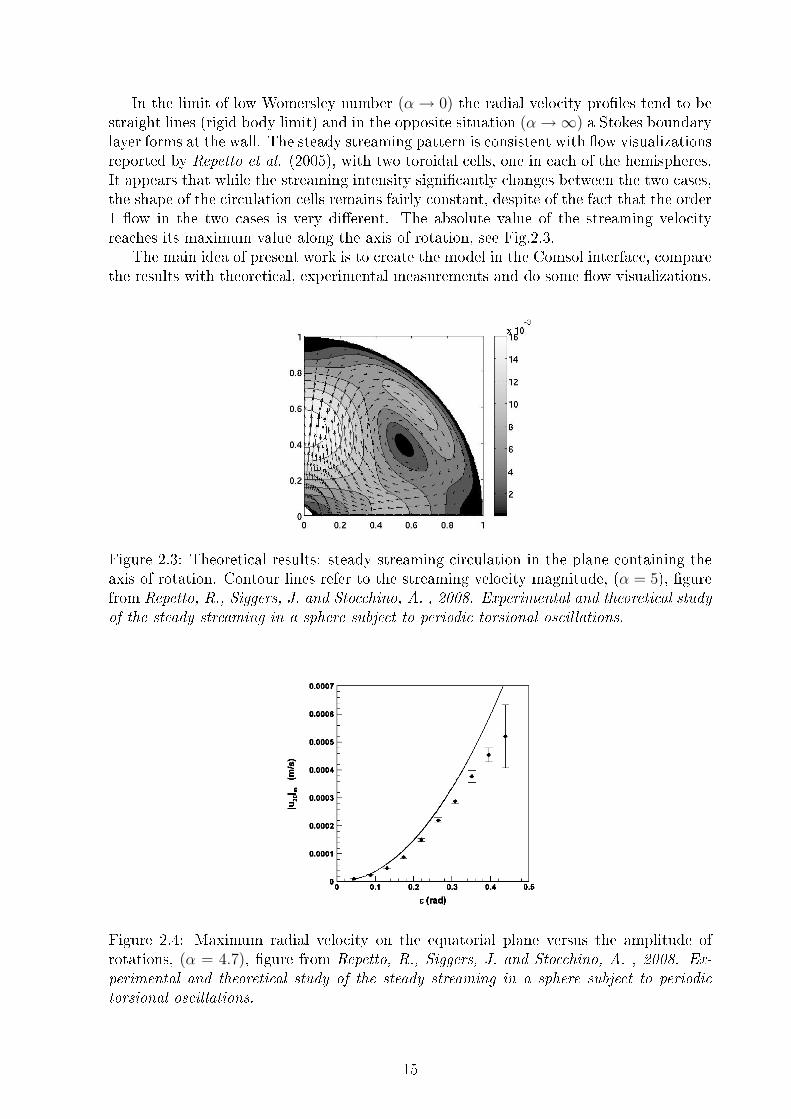
In the limit of low Womersley number (α→ 0) the radial velocity proles tend to bestraight lines (rigid body limit) and in the opposite situation (α→∞) a Stokes boundarylayer forms at the wall. The steady streaming pattern is consistent with ow visualizationsreported by Repetto et al. (2005), with two toroidal cells, one in each of the hemispheres.It appears that while the streaming intensity signicantly changes between the two cases,the shape of the circulation cells remains fairly constant, despite of the fact that the order1 ow in the two cases is very dierent. The absolute value of the streaming velocityreaches its maximum value along the axis of rotation, see Fig.2.3.
The main idea of present work is to create the model in the Comsol interface, comparethe results with theoretical, experimental measurements and do some ow visualizations.
Figure 2.3: Theoretical results: steady streaming circulation in the plane containing theaxis of rotation. Contour lines refer to the streaming velocity magnitude, (α = 5), gurefrom Repetto, R., Siggers, J. and Stocchino, A. , 2008. Experimental and theoretical studyof the steady streaming in a sphere subject to periodic torsional oscillations.
Figure 2.4: Maximum radial velocity on the equatorial plane versus the amplitude ofrotations, (α = 4.7), gure from Repetto, R., Siggers, J. and Stocchino, A. , 2008. Ex-perimental and theoretical study of the steady streaming in a sphere subject to periodictorsional oscillations.
15
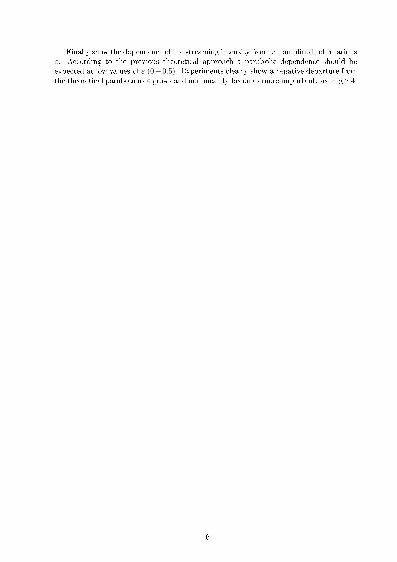
Finally show the dependence of the streaming intensity from the amplitude of rotationsε. According to the previous theoretical approach a parabolic dependence should beexpected at low values of ε (0−0.5). Experiments clearly show a negative departure fromthe theoretical parabola as ε grows and nonlinearity becomes more important, see Fig.2.4.
16
Chapter 3
Finite Element Method, Comsol
3.1 FEM
3.1.1 An Introduction to the Finite Element Method
Analytical descriptions of physical phenomena and processes are calledmathematical mod-els. Mathematical models of a process are developed using assumptions concerning howthe process works and using appropriate axioms or laws governing the process, and theyare often characterized by very complex dierential or integral equations posed on geo-metrically complicated domains. Over the last three decades, however, computers havemade it possible, with the help of suitable mathematical models and numerical methods,to solve many practical problems of engineering. The use of a numerical method and acomputer to evaluate the mathematical model of a process and estimate its characteristicsis called a numerical simulation.
Any numerical simulation, such as the one by the nite element method, is not an endin itself but rather an aid to design and manufacturing. There are several reasons whyan engineer or scientist should study a numerical method, especially the nite elementmethod :
1) Most practical problems involve complicated domains (both geometry and materialconstitution), loads, and nonlinearities that forbid the development of analytical solutions.Therefore, the only alternative is to nd approximate solutions using numerical methods.
2) A numerical method, with the advent of a computer, can be used to investigate theeects of various parameters (e.g., geometry, material parameters, or loads) of the systemon its response to gain a better understanding of the process being analyzed. It is moreeective and saves time.
3) Because of the power of numerical methods and electronic computation, it is possi-ble to include all relevant features in a mathematical model of a physical process withoutworrying about its solution by exact means.
4) Those who are quick to use a computer program rather than think about the prob-lem to be analyzed may nd it dicult to interpret or explain the computer-generatedresults.
5) The nite element method and its generalizations are the most powerful computer-
17
oriented methods ever devised to analyze practical engineering problems. Today, niteelement analysis is an integral and major component in many elds of engineering designand manufacturing.
3.2 Mathematical Models
A mathematical model can be broadly dened as a set of equations that expresses theessential features of a physical system in terms of variables that describe the system.The mathematical models of physical phenomena are often based on fundamental scien-tic laws of physics such as the principle of conservation of mass, conservation of linearmomentum, and conservation of energy.
3.3 Numerical Simulations
By a numerical simulation of a process, we mean the solution of the governing equationsof the process using a numerical method and a computer. Numerical methods typicallytransform dierential equations governing a continuum to a set of algebraic equations ofa discrete model of the continuum that are to be solved using computers.
There exist a number of numerical methods, many of which are developed to solvedierential equations. In the nite dierence approximation of a dierential equation, thederivatives in the latter are replaced by dierence quotients (or the function is expandedin a Taylor series) that involve the values of the solution at discrete mesh points of thedomain. The resulting algebraic equations are solved for the values of the solution at themesh points after imposing the boundary conditions.
In the solution of a dierential equation by a classical variational method, the equa-tion is put into an equivalent weighted-integral form and then the approximate solutionover the domain is assumed to be a linear combination
∑j cjφj of appropriately chosen
approximation functions φj and undetermined coecients cj. The coecients cj are de-termined such that the integral statement equivalent to the original dierential equationis satised. The classical variational methods, which are truly meshless methods, are pow-erful methods that provide globally continuous solutions but suer from the disadvantagethat the approximation functions for problems with arbitrary domains are dicult to con-struct (the modern meshless methods seem to provide a way to construct approximationfunctions for arbitrary domains).
3.4 The Finite Element Method
3.4.1 The Basic Idea
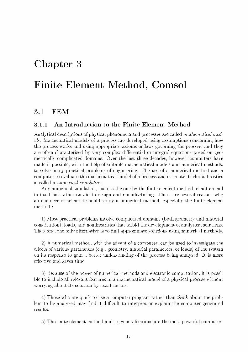
The nite element method is a numerical method like the nite dierence method but ismore general and powerful in its application to real-world problems that involve compli-cated physics, geometry, and boundary conditions. In the nite element method, a givendomain is viewed as a collection of subdomains, and over each subdomain the governingequation is approximated by any of the traditional variational methods. The main reasonbehind seeking approximate solution on a collection of subdomains is the fact that it iseasier to represent a complicated function as collection of simple polynomials, as can beseen from see Fig.3.1. Of course, each individual segment of the solution should t with
18
its neighbors in the sense that the function and possibly derivatives up to a chosen orderare continuous at the connecting points.
Figure 3.1: Piecewise approximation of a function
3.4.2 The Basic Features
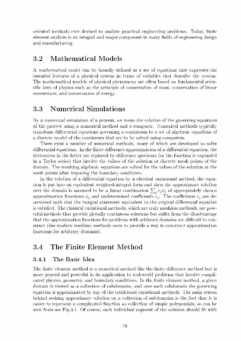
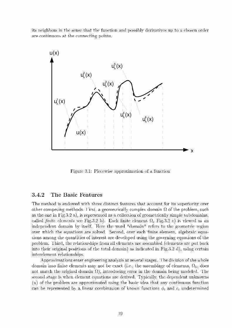
The method is endowed with three distinct features that account for its superiority overother competing methods. First, a geometrically complex domain Ω of the problem, suchas the one in Fig.3.2 a), is represented as a collection of geometrically simple subdomains,called nite elements see Fig.3.2 b). Each nite element Ωe Fig.3.2 c) is viewed as anindependent domain by itself. Here the word "domain" refers to the geometric regionover which the equations are solved. Second, over each nite element, algebraic equa-tions among the quantities of interest are developed using the governing equations of theproblem. Third, the relationships from all elements are assembled (elements are put backinto their original positions of the total domain) as indicated in Fig.3.2 d), using certaininterelement relationships.
Approximations enter engineering analysis at several stages. The division of the wholedomain into nite elements may not be exact (i.e., the assemblage of elements, Ωh, doesnot match the original domain Ω), introducing error in the domain being modeled. Thesecond stage is when element equations are derived. Typically, the dependent unknowns(u) of the problem are approximated using the basic idea that any continuous functioncan be represented by a linear combination of known functions φi and ci undetermined
19
Figure 3.2: Representation of a two-dimensional domain by a collection of triangles andquadrilaterals.
coecients.
(u ≈ uh =n∑i=0
ciφi)
Algebraic relations among the undetermined coecients cj are obtained by satisfying thegoverning equations, in a weighted-integral sense, over each element. The approximationfunctions φi are often taken to be polynomials, and they are derived using conceptsfrom interpolation theory. Therefore, they are termed interpolation functions. Thusapproximation errors in the second stage are introduced both in representing the solutionu as well as in evaluating the integrals. Finally, errors are introduced in solving theassembled system of equations. Obviously, some of the errors discussed above can bezero. When all the errors are zero, we obtain the exact solution of the problem (which isnot the case in most problems).
3.4.3 Simple Example
Let us consider the simple problem of determining the perimeter of a circle of radius Rsee Fig.3.3 a). We pretend that we don't know the formula (P = 2πR) for the perimeterof a circle. Ancient mathematicians estimated the value of the perimeter of a circle byapproximating it by (straight) line segments, whose lengths they were able to measure.The approximate value of the perimeter is obtained by summing the lengths of the linesegments used to represent it.
The three basic features of the nite element method in the present case take thefollowing form. First, the division of the perimeter of a circle into a collection of linesegments. In theory, we need an innite number of such line elements to represent the
20
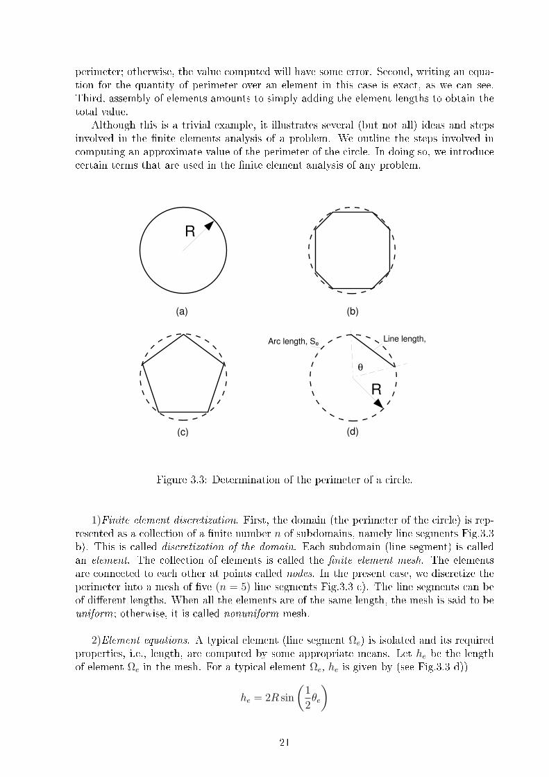
perimeter; otherwise, the value computed will have some error. Second, writing an equa-tion for the quantity of perimeter over an element in this case is exact, as we can see.Third, assembly of elements amounts to simply adding the element lengths to obtain thetotal value.
Although this is a trivial example, it illustrates several (but not all) ideas and stepsinvolved in the nite elements analysis of a problem. We outline the steps involved incomputing an approximate value of the perimeter of the circle. In doing so, we introducecertain terms that are used in the nite element analysis of any problem.
Figure 3.3: Determination of the perimeter of a circle.
1)Finite element discretization. First, the domain (the perimeter of the circle) is rep-resented as a collection of a nite number n of subdomains, namely line segments Fig.3.3b). This is called discretization of the domain. Each subdomain (line segment) is calledan element. The collection of elements is called the nite element mesh. The elementsare connected to each other at points called nodes. In the present case, we discretize theperimeter into a mesh of ve (n = 5) line segments Fig.3.3 c). The line segments can beof dierent lengths. When all the elements are of the same length, the mesh is said to beuniform; otherwise, it is called nonuniform mesh.
2)Element equations. A typical element (line segment Ωe) is isolated and its requiredproperties, i.e., length, are computed by some appropriate means. Let he be the lengthof element Ωe in the mesh. For a typical element Ωe, he is given by (see Fig.3.3 d))
he = 2R sin
(1
2θe
)
21
where R is the radius of the circle and θe < π is the angle subtended by the line segment.The above equations are called element equations.
3) Assembly of element equations and solution. The approximate value of the perimeterof the circle is obtained by putting together the element properties in a meaningful way;this process is called the assembly of the element equations. It is based, in the presentcase, on the simple idea that the total perimeter of the polygon Ωh is equal to the sum ofthe lengths of individual elements :
Pn =n∑e=1
he
Then Pn represents an approximation to the actual perimeter, P . If the mesh is uniform,or he is the same for each of the elements in the mesh, then θe = 2π/n, and we have
Pn = n(
2R sinπ
n
)4) Convergence and error estimate. For this simple problem, we know the exact solution :P = 2πR. We can estimate the error in the approximation and show that the approximatesolution Pn converges to the exact value P in the limit as n → ∞. Consider a typicalelement Ωe. The error in the approximation is equal to the dierence between the lengthof the sector and that of the line segment.(Fig.3.3 d))
Ee = |Se − he|
where Se = Rθe is the length of the sector. Thus, the error estimate for an element in themesh is given by
Ee = R ·(
2π
n− 2 sin
π
n
)The total error (called global error) is given by multiplying Ee by n :
E = nEe = 2R(π − n sin
π
n
)= 2πR− Pn = P − Pn
We now show that E goes to zero as n→∞. Letting x = 1/n, we have
Pn = 2Rn sinπ
n= 2R
sinπx
x
and
limn→∞
Pn = limx→0
(2R
sin πx
x
)= lim
x→0
(2πR
cos πx
1
)= 2πR
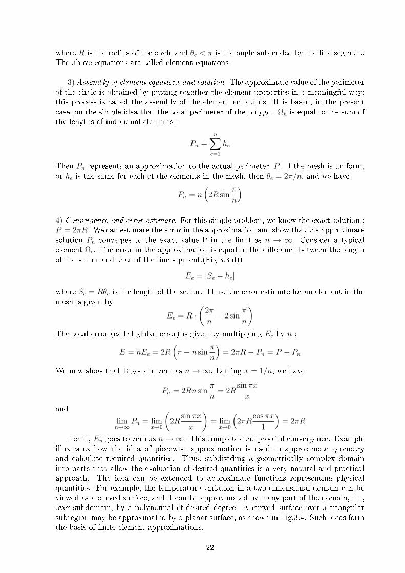
Hence, En goes to zero as n→∞. This completes the proof of convergence. Exampleillustrates how the idea of piecewise approximation is used to approximate geometryand calculate required quantities. Thus, subdividing a geometrically complex domaininto parts that allow the evaluation of desired quantities is a very natural and practicalapproach. The idea can be extended to approximate functions representing physicalquantities. For example, the temperature variation in a two-dimensional domain can beviewed as a curved surface, and it can be approximated over any part of the domain, i.e.,over subdomain, by a polynomial of desired degree. A curved surface over a triangularsubregion may be approximated by a planar surface, as shown in Fig.3.4. Such ideas formthe basis of nite element approximations.
22
Figure 3.4: Approximation of a curved surface by a planar surface
3.4.4 Some Remarks
In the nite element method a given domain is divided into subdomains, called niteelements, and an approximate solution to the problem is developed over each element.The subdivision of a whole domain into parts has two advantages:
1) Allows accurate representation of complex geometry and inclusion of dissimilar ma-terial properties.
2) Enables easy representation of the total solution by functions dened within eachelement that capture local eects.
3.4.5 Summary
In a numerical simulation of physical processes, we employ a numerical method and com-puter to evaluate the mathematical model of the process. The nite element method is apowerful numerical method of solving algebraic, dierential, and integral equations, andit is devised to study complex physical processes. The method is characterized by threefeatures :
1) The domain of the problem is represented by a collection of simple subdomains,called nite elements. The collection of nite elements is called the nite element mesh.
2) Over each nite element, the physical process is approximated by functions of thedesired type (polynomial or otherwise), and algebraic equations relating physical quanti-ties at selective points, called nodes, of the element are developed.
3) The element equations are assembled using continuity and "balance" of physicalquantities.
23
In the nite element method, we seek an approximation uh of u in the form
u ≈ uh =n∑j=1
ujψj +m∑j=1
cjφj
where uj are the values of uh at the elements nodes, φj are the interpolation functions, cjare coecients that are not associated with nodes, and φ are the associated approximationfunctions.
There is only one method of nite elements that is characterized by the three featuresstated above. Of course, there can be more than one nite element model of the sameproblem. The type of model depends on the dierential equations, methods used toderive the algebraic equations (i.e., the weighted-integral form used) for the undeterminedcoecients over an element, and nature of the approximation functions used. It is obviousthese statements written above give you just the basic idea of the nite element method,there are several other features that are not present or not apparent. Main purpose of thissection is to be more familiar with idea of FEM. This numerical method is used in ComsolMultiphysics which is well known simulation software for evaluating the mathematicalmodel of a process.
3.5 What is COMSOL
COMSOL Multiphysics is a modeling package for the simulation of any physical processyou can describe with partial dierential equations (PDEs). You can easily model mostphenomena through predened modeling templates. Modifying these to specic applica-tions is possible through equation-based modeling capabilities. To deal with the increasingdemand for realistic representations of the world around us, you can easily model systemsof coupled physics phenomena. It provides a friendly, fast and versatile environment formultiphysics modeling. The simulation environment facilitates all steps in the modelingprocess - dening your geometry, specifying your physics, meshing, solving and then post-processing your results. If you are using library contains models than model set up canbe quick, thanks to a number of predened modeling interfaces for applications rangingfrom uid ow and heat transfer to structural mechanics and electromagnetic analysis.Material properties, source terms and boundary conditions can all be arbitrary functionsof the dependent variables. So by using model library multiphysics simulation can beachieved in minutes. Predened multiphysics-application templates solve many commonproblem types. You as the user, also have the option of choosing dierent physics fromthe Multiphysics menu and dening the interdependencies yourself. Or you can specifyyour own Partial Dierential Equations (PDEs), and couple them with other equationsand physics. Any number of PDEs can be automatically coupled with any others, irre-spective of the application area. This makes COMSOL for simulating cross-disciplinaryapplications or traditional engineering elds aected by other physics. All models can beaccessed as a script and then manipulated, run, and controlled from the COMSOL Scriptor MATLAB command line.
24
Chapter 4
Formulation of the Problem
4.1 Introduction
We model numerically the motion of the liqueed vitreous within the vitreous cavityinduced by dierent eye movements. In order to formulate the appropriate mathematicalmodel we set down as much informations as possible regarding the natural movement ofthe eye.
This clearly occurs during what is known as saccadic motion, similar to the movementof the eye from left to right and back again when reading this thesis. Weber and Daro(1972) in their experiments on rexation saccades show the eye velocity to be of sine form.
We shall for this analysis treat the vitreous as a Newtonian incompressible uid. Asdiscussed in the rst chapter, this applies to the case of liqueed vitreous or to the casein which the vitreous chamber is lled with aqueous humour after surgery. The humaneyeglobe is thought of as a thin-shelled sphere of internal radius, R0 and it's rotatingabout its vertical axis. This model is ideal, because we describe the vitreous chamber as asphere. Recently Repetto (2006) and Stocchino et al (2007) have shown that an even smalldeparture from the spherical shape might have important hydrodynamic consequences onthe ow eld. Moreover we consider a Newtonian uid and rotations only about thevertical axis. As we see later these conditions allow to model the problem just in 2Dinstead of 3D.
4.2 Equations in Cylindrical Coordinates
4.2.1 Coordinate system
First we need to dene the system of equations in the weak form which govern the owwithin the sphere induced by its rotation. We will see later that the weak form is moreuseful in the Comsol interface. The mathematical model is formulated referring to an os-cillating sphere about its vertical axis and employing a system of cylindrical coordinates.
The cylindrical coordinate system (r, θ, z) is a three-dimensional coordinate systemwhich essentially extends circular polar coordinates by adding a third coordinate (usu-ally denoted z) which measures the height of a point above the plane. The notation forthis coordinate system is not uniform because in many cases the azimuthal coordinate θis denoted as ϕ. Also, the radial coordinate is sometimes called ρ while the vertical issometimes referred to as h.
25
P
Oyx
yr
z
z
r
(r, ,z)
z
x
P'
Figure 4.1: The eye represents by a sphere in the cylindrical coordinates
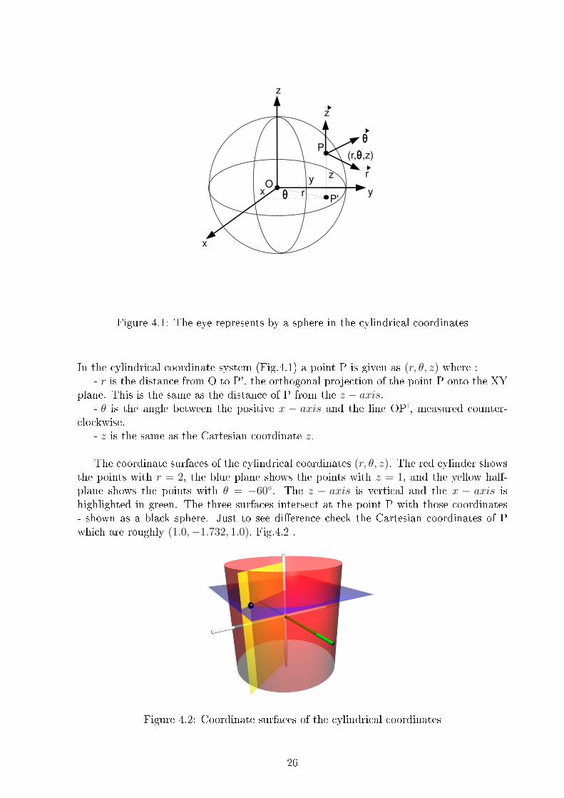
In the cylindrical coordinate system (Fig.4.1) a point P is given as (r, θ, z) where :- r is the distance from O to P', the orthogonal projection of the point P onto the XY
plane. This is the same as the distance of P from the z − axis.- θ is the angle between the positive x − axis and the line OP', measured counter-
clockwise.- z is the same as the Cartesian coordinate z.
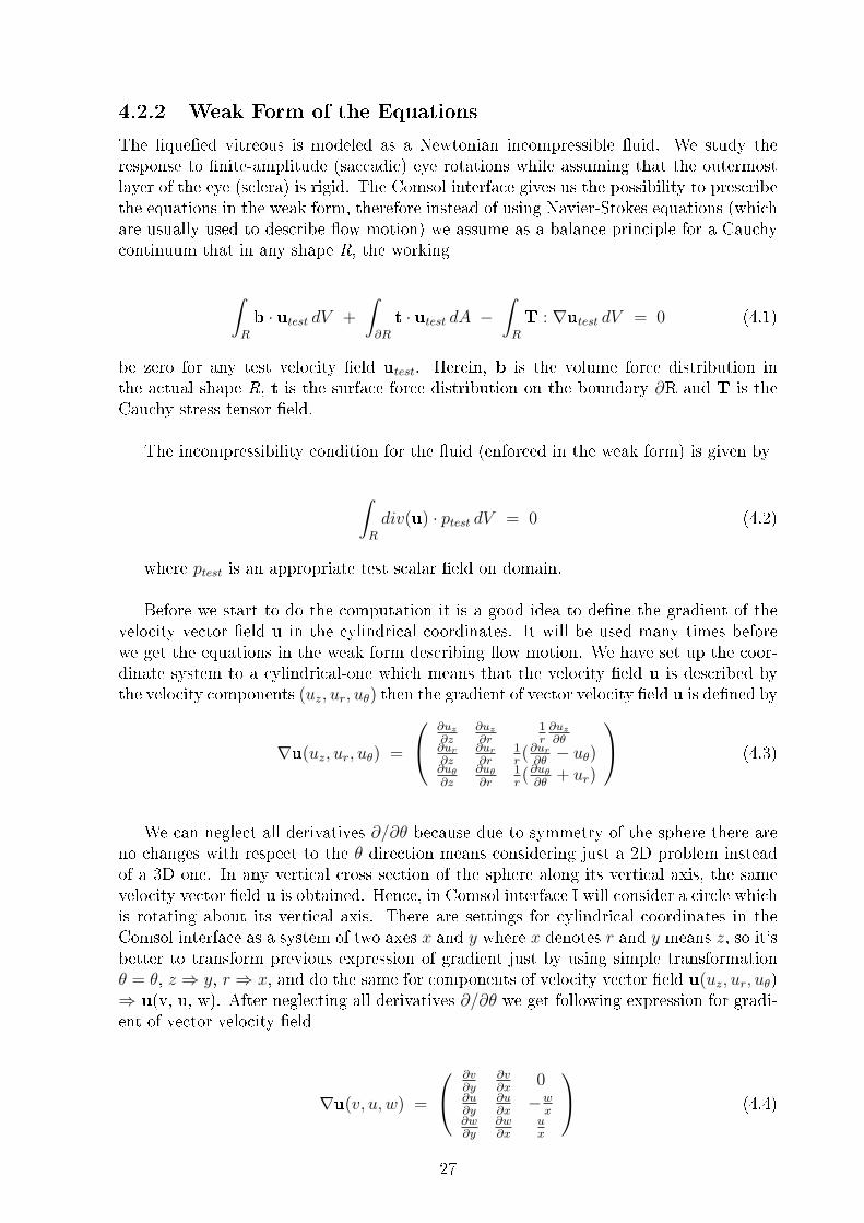
The coordinate surfaces of the cylindrical coordinates (r, θ, z). The red cylinder showsthe points with r = 2, the blue plane shows the points with z = 1, and the yellow half-plane shows the points with θ = −60. The z − axis is vertical and the x − axis ishighlighted in green. The three surfaces intersect at the point P with those coordinates- shown as a black sphere. Just to see dierence check the Cartesian coordinates of Pwhich are roughly (1.0,−1.732, 1.0), Fig.4.2 .
Figure 4.2: Coordinate surfaces of the cylindrical coordinates
26
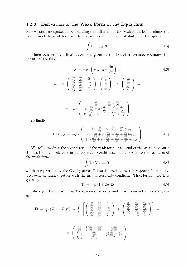
4.2.2 Weak Form of the Equations
The liqueed vitreous is modeled as a Newtonian incompressible uid. We study theresponse to nite-amplitude (saccadic) eye rotations while assuming that the outermostlayer of the eye (sclera) is rigid. The Comsol interface gives us the possibility to prescribethe equations in the weak form, therefore instead of using Navier-Stokes equations (whichare usually used to describe ow motion) we assume as a balance principle for a Cauchycontinuum that in any shape R, the working
∫R
b · utest dV +
∫∂R
t · utest dA −∫R
T : ∇utest dV = 0 (4.1)
be zero for any test velocity eld utest. Herein, b is the volume force distribution inthe actual shape R, t is the surface force distribution on the boundary ∂R and T is theCauchy stress tensor eld.
The incompressibility condition for the uid (enforced in the weak form) is given by
∫R
div(u) · ptest dV = 0 (4.2)
where ptest is an appropriate test scalar eld on domain.
Before we start to do the computation it is a good idea to dene the gradient of thevelocity vector eld u in the cylindrical coordinates. It will be used many times beforewe get the equations in the weak form describing ow motion. We have set up the coor-dinate system to a cylindrical-one which means that the velocity eld u is described bythe velocity components (uz, ur, uθ) then the gradient of vector velocity eld u is dened by
∇u(uz, ur, uθ) =
∂uz∂z
∂uz∂r
1r∂uz∂θ
∂ur∂z
∂ur∂r
1r(∂ur∂θ− uθ)
∂uθ∂z
∂uθ∂r
1r(∂uθ∂θ
+ ur)
(4.3)
We can neglect all derivatives ∂/∂θ because due to symmetry of the sphere there areno changes with respect to the θ direction means considering just a 2D problem insteadof a 3D one. In any vertical cross section of the sphere along its vertical axis, the samevelocity vector eld u is obtained. Hence, in Comsol interface I will consider a circle whichis rotating about its vertical axis. There are settings for cylindrical coordinates in theComsol interface as a system of two axes x and y where x denotes r and y means z, so it'sbetter to transform previous expression of gradient just by using simple transformationθ = θ, z ⇒ y, r ⇒ x, and do the same for components of velocity vector eld u(uz, ur, uθ)⇒ u(v, u, w). After neglecting all derivatives ∂/∂θ we get following expression for gradi-ent of vector velocity eld
∇u(v, u, w) =
∂v∂y
∂v∂x
0∂u∂y
∂u∂x−w
x∂w∂y
∂w∂x
ux
(4.4)
27
4.2.3 Derivation of the Weak Form of the Equations
Now we start computation by following the denition of the weak form, let's evaluate therst term of the weak form which represents volume force distribution in the sphere.∫
R
b · utest dV (4.5)
where volume force distribution b is given by the following formula, ρ denotes thedensity of the uid
b = −ρ ·(∇u · u +
∂u
∂t
)= (4.6)
= −ρ ·
∂v∂y
∂v∂x
0∂u∂y
∂u∂x−w
x∂w∂y
∂w∂x
ux
· v
uw
− ρ · ∂v
∂t∂u∂t∂w∂t
=
= −ρ ·
v · ∂v∂y
+ u · ∂v∂x
+ ∂v∂t
v · ∂u∂y
+ u · ∂u∂x− w2
x+ ∂u
∂t
v · ∂w∂y
+ u · ∂w∂x
+ w·ux
+ ∂w∂t
so nally
b · utest = −ρ ·
(v · ∂v∂y
+ u · ∂v∂x
+ ∂v∂t
)vtest
(v · ∂u∂y
+ u · ∂u∂x− w2
x+ ∂u
∂t)utest
(v · ∂w∂y
+ u · ∂w∂x
+ w·ux
+ ∂w∂t
)wtest
(4.7)
We will introduce the second term of the weak form at the end of this section becauseit plays the main role only in the boundary conditions. So let's evaluate the last term ofthe weak form ∫
R
T · ∇utest dV (4.8)
which is represents by the Cauchy stress T that is provided by the response function fora Newtonian uid, together with the incompressibility condition. Then formula for T isgiven by
T = −p · I + 2µ0D (4.9)
where p is the pressure, µ0 the dynamic viscosity and D is a symmetric matrix givenby
D = 12· (∇u +∇uT ) = 1
2·
∂v∂y
∂v∂x
0∂u∂y
∂u∂x−w
x∂w∂y
∂w∂x
ux
+
∂v∂y
∂u∂y
∂w∂y
∂v∂x
∂u∂x
∂w∂x
0 −wx
ux
=
=
∂v∂y
12( ∂v∂x
+ ∂u∂y
) 12∂w∂y
D12∂u∂x
12(∂w∂x− w
x)
D13 D23ux
28
using expression above we can write Cauchy stress tensor eld as a matrix
T =
−p 0 00 −p 00 0 −p
+
2µ0∂v∂y
µ0(∂v∂x
+ ∂u∂y
) µ0∂w∂y
2µ0D12 2µ0∂u∂x
µ0(∂w∂x− w
x)
2µ0D13 2µ0D23 2µ0ux
=
=
−p+ 2µ0∂v∂y
µ0(∂v∂x
+ ∂u∂y
) µ0∂w∂y
t12 −p+ 2µ0∂u∂x
µ0(∂w∂x− w
x)
t13 t23 −p+ 2µ0ux
and nally we can write
T : ∇utest =
=
−p+ 2µ0∂v∂y
µ0(∂v∂x
+ ∂u∂y
) µ0∂w∂y
t12 −p+ 2µ0∂u∂x
µ0(∂w∂x− w
x)
t13 t23 −p+ 2µ0ux
:
∂vtest∂y
∂vtest∂x
0∂utest∂y
∂utest∂x
−wtestx
∂wtest∂y
∂wtest∂x
utestx
=
=
(−p+ 2µ0∂v∂y
)∂vtest∂y
µ0(∂v∂x
+ ∂u∂y
)∂vtest∂x
0
t12∂utest∂y
(−p+ 2µ0∂u∂x
)∂utest∂x
−µ0(∂w∂x− w
x)wtest
x
t13∂wtest∂y
t23∂wtest∂x
(−p+ 2µ0ux)utest
x
(4.10)
By putting terms (4.7) and (4.10) together we obtain a equation (which can be splitinto three equations) in the weak form which describes the ow motion. These equationscan be used to model exactly the problem with relevant values of ρ, µ0, ε, ω0 and R0. Wecan use them in the Comsol-environment exactly in the form reported below. For ourinvestigation is better to reduce the number of such controlling parameters.
−ρ ·(v · ∂v
∂y+ u · ∂v
∂x+∂v
∂t
)· vtest − t11 ·
∂vtest∂y− t12 ·
∂vtest∂x
= 0
−ρ ·(v · ∂u
∂y+ u · ∂u
∂x− w2
x+∂u
∂t
)· utest − t12 ·
∂utest∂y
− t22 ·∂utest∂x
+ t23 ·wtestx
= 0
−ρ ·(v · ∂w
∂y+ u · ∂w
∂x+w · ux
+∂w
∂t
)· wtest − t13 ·
∂wtest∂y
− t23 ·∂wtest∂x
− t33 ·utestx
= 0
where :
t11 = −p+ 2µ0∂v
∂yt12 = µ0
(∂v
∂x+∂u
∂y
)t13 = µ0
∂w
∂y
t22 = −p+ 2µ0∂u
∂xt23 = µ0
(∂w
∂x− w
x
)t33 = −p+ 2µ0
u
x
29
4.2.4 Boundary and Incompressibility Conditions
Motion of the vitreous is induced by saccades. Saccadic motion, which is a single rapidrotation of the eye, is adequately modelled by choosing the sphere to move sinusoidallywith frequency ω0 and amplitude ε.
Movement of the outer most layer of the sphere, is described as a harmonic motion byequation of deviation x(t) :
x(t) = −ε cos(ω0t+ ϕ) (4.11)
where ε, ω0 and ϕ are constants such that ε is a positive constant representing the maxi-mum possible deviation, usually is called the amplitude, ϕ represents initial deviation att = 0 and ω0 as the angular frequency (also referred to by the terms angular speed, radialfrequency, circular frequency, and radian frequency) is a scalar measure of rotation rateand is measured in radians per second. To obtain the expression for the velocity of theharmonic motion we just dierentiate the previous equation (4.11).
v(t) =dx
dt=
d
dt(−ε cos(ω0t+ ϕ)) = ω0ε sin(ω0t+ ϕ) (4.12)
To get the velocity component w we multiply v(t) by radius r (r ⇒ x), nally we canwrite boundary conditions at the wall as follows :
u = 0, v = 0, w = ε · ω0 · sin(t · ω0) · x (4.13)
At the end we assign the incompressibility condition for the uid, which from (4.2) isgiven by
div(u) · ptest = trace(∇u) · ptest =
(∂v
∂y+∂u
∂x+u
x
)· ptest = 0 (4.14)
4.2.5 Dimensionless Form of the Governing Equation
We would like to investigate the dependence of the solution on the controlling parameters,so the best we can do, is to use scaling and reduce the number of parameters. Themain purpose is to determine the dependence of the steady streaming intensity on suchparameters. We adopt the following scaling for the velocity u, the time t, the pressure pand the coordinates x and y.
u∗ =u
ε2 · ω0 ·R0
, v∗ =v
ε2 · ω0 ·R0
, w∗ =w
ε · ω0 ·R0
, x∗ =x
R0
,
y∗ =y
R0
, t∗ = t · ω0 , p∗ =p
ε · µ0 · ω0
where superscript star indicate dimensionless variable. Note than u and v are scaleddierently with respect to w. The opportunity of such a choice is suggested by thetheoretical work of Repetto et al. (2008) which show that in the perturbation solution wrst appears at order 1 while u and v at order 2.
30
First we apply scaling on the gradient and we get following expression
∇u(v, u, w) =
∂v∂y
∂v∂x
0∂u∂y
∂u∂x−w
x∂w∂y
∂w∂x
ux
=
=
ε2ω0R0 · ∂v∗
∂y∗∂y∗
∂yε2ω0R0 · ∂v
∗
∂x∗∂x∗
∂x0
ε2ω0R0 · ∂u∗
∂y∗∂y∗
∂yε2ω0R0 · ∂u
∗
∂x∗∂x∗
∂xεω0R0 · (− w∗
x∗R0)
εω0R0 · ∂w∗
∂y∗∂y∗
∂yεω0R0 · ∂w
∗
∂x∗∂x∗
∂xε2ω0R0 · u∗
x∗R0
=
=
ε2ω0R0 · ∂v∗
∂y∗1R0
ε2ω0R0 · ∂v∗
∂x∗1R0
0
ε2ω0R0 · ∂u∗
∂y∗1R0
ε2ω0R0 · ∂u∗
∂x∗1R0
εω0R0 · (− w∗
x∗R0)
εω0R0 · ∂w∗
∂y∗1R0
εω0R0 · ∂w∗
∂x∗1R0
ε2ω0R0 · u∗
x∗R0
=
= ω0 ·
ε2 · ∂v∗∂y∗
ε2 · ∂v∗∂x∗
0
ε2 · ∂u∗∂y∗
ε2 · ∂u∗∂x∗
ε · (−w∗
x∗)
ε · ∂w∗
∂y∗ε · ∂w∗
∂x∗ε2 · u∗
x∗
Let's apply scaling on the rst term of the weak form. As before we rst evaluate the
expression of volume force distribution b given by
b = −ρ ·(∇u · u +
∂u
∂t
)=
= −ρω0 ·
ε2 · ∂v∗∂y∗
ε2 · ∂v∗∂x∗
0
ε2 · ∂u∗∂y∗
ε2 · ∂u∗∂x∗
ε · (−w∗
x∗)
ε · ∂w∗
∂y∗ε · ∂w∗
∂x∗ε2 · u∗
x∗
v · ε2ω0R0
u · ε2ω0R0
w · εω0R0
− ρ ε2ω0R0
∂v∗
∂t∗∂t∗
∂t
ε2ω0R0∂u∗
∂t∗∂t∗
∂t
εω0R0∂w∗
∂t∗∂t∗
∂t
=
= −ρω20R0 ·
ε4 · v∗ · ∂v∗∂y∗
+ ε4 · u∗ · ∂v∗∂x∗
+ ε2 · ∂v∗∂t∗
ε4 · v∗ · ∂u∗∂y∗
+ ε4 · u∗ · ∂u∗∂x∗− ε2 · w∗2
x∗+ ε2 · ∂u∗
∂t∗
ε3 · v∗ · ∂w∗
∂y∗+ ε3 · u∗ · ∂w∗
∂x∗+ ε3 · w∗·u∗
x∗+ ε · ∂w∗
∂t∗
By using the above expression we get
b · utest =
= −ρω20R0
ε4 · v∗ · ∂v∗∂y∗
+ ε4 · u∗ · ∂v∗∂x∗
+ ε2 · ∂v∗∂t∗
ε4 · v∗ · ∂u∗∂y∗
+ ε4 · u∗ · ∂u∗∂x∗− ε2 · w∗2
x∗+ ε2 · ∂u∗
∂t∗
ε3 · v∗ · ∂w∗
∂y∗+ ε3 · u∗ · ∂w∗
∂x∗+ ε3 · w∗·u∗
x∗+ ε · ∂w∗
∂t∗
· ε2ω0R0 · v∗test
ε2ω0R0 · u∗testεω0R0 · w∗test
=
= −ρω30R
20 ·
ε6 · v∗ · ∂v∗∂y∗
+ ε6 · u∗ · ∂v∗∂x∗
+ ε4 · ∂v∗∂t∗
ε6 · v∗ · ∂u∗∂y∗
+ ε6 · u∗ · ∂u∗∂x∗− ε4 · w∗2
x∗+ ε4 · ∂u∗
∂t∗
ε4 · v∗ · ∂w∗
∂y∗+ ε4 · u∗ · ∂w∗
∂x∗+ ε4 · w∗·u∗
x∗+ ε2 · ∂w∗
∂t∗
· u∗test(4.15)
31
Again we apply the scaling on the last term of the weak form, but rst computeCauchy stress tensor eld
T = −p · I + 2µ0D
where D is a symmetric matrix
D = 12· (∇u +∇uT ) = 1
2·
∂v∂y
∂v∂x
0∂u∂y
∂u∂x−w
x∂w∂y
∂w∂x
ux
+
∂v∂y
∂u∂y
∂w∂y
∂v∂x
∂u∂x
∂w∂x
0 −wx
ux
=
= 12·
ω0 ·
ε2 · ∂v∗∂y∗
ε2 · ∂v∗∂x∗
0
ε2 · ∂u∗∂y∗
ε2 · ∂u∗∂x∗
ε · (−w∗
x∗)
ε · ∂w∗
∂y∗ε · ∂w∗
∂x∗ε2 · u∗
x∗
+ ω0 ·
ε2 · ∂v∗∂y∗
ε2 · ∂u∗∂y∗
ε · ∂w∗
∂y∗
ε2 · ∂v∗∂x∗
ε2 · ∂u∗∂x∗
ε · ∂w∗
∂x∗
0 −ε · w∗
x∗ε2 · u∗
x∗
=
=
ε2 · ω0 · ∂v∗
∂y∗ε2 · ω0 · 1
2· ( ∂v∗
∂x∗+ ∂u∗
∂y∗) ε · ω0 · 1
2∂w∗
∂y∗
D12 ε2 · ω0 · ∂u∗
∂x∗ε · ω0 · 1
2(∂w
∗
∂x∗− w∗
x∗)
D13 D23 ε2 · ω0 · u∗
x∗
Now we can write Cauchy stress tensor eld as a matrix
T = εµ0ω0(−p∗) + ε2 · 2µ0ω0∂v∗
∂y∗ε2 · µ0ω0(
∂v∗
∂x∗+ ∂u∗
∂y∗) ε · µ0ω0
∂w∗
∂y∗
t12 εµ0ω0(−p∗) + ε2 · 2µ0ω0∂u∗
∂x∗ε · µ0ω0(
∂w∗
∂x∗− w∗
x∗)
t13 t23 εµ0ω0(−p∗) + ε2 · 2µ0ω0u∗
x∗
so nally we obtain
T : utest = εµ0ω0(−p∗) + ε2 · 2µ0ω0∂v∗
∂y∗ε2 · µ0ω0(
∂v∗
∂x∗+ ∂u∗
∂y∗) ε · µ0ω0
∂w∗
∂y∗
t12 εµ0ω0(−p∗) + ε2 · 2µ0ω0∂u∗
∂x∗ε · µ0ω0(
∂w∗
∂x∗− w∗
x∗)
t13 t23 εµ0ω0(−p∗) + ε2 · 2µ0ω0u∗
x∗
:
:
ε2 · ∂v∗test
∂y∗ε2 · ∂v
∗test
∂x∗0
ε2 · ∂u∗test
∂y∗ε2 · ∂u
∗test
∂x∗ε · (−w∗
test
x∗)
ε · ∂w∗test
∂y∗ε · ∂w
∗test
∂x∗ε2 · u
∗test
x∗
· ω0
(4.16)
We dene the dimensionless parameter α, named the Womersley number, as
α =
√ω0 ·R2
0
ν0
(4.17)
where R0 denotes the radius of the sphere and ν0 is the kinematic viscosity of the uid.The importance of such a dimensionless group, characterize unsteady internal ows is
32
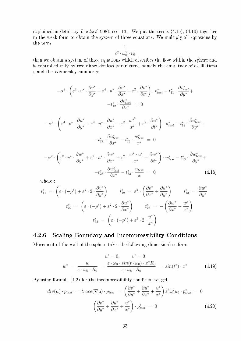
explained in detail by Loudon(1998), see [13]. We put the terms (4.15), (4.16) togetherin the weak form to obtain the system of three equations. We multiply all equations bythe term
1
ε2 · ω20 · ν0
then we obtain a system of three equations which describes the ow within the sphere andis controlled only by two dimensionless parameters, namely the amplitude of oscillationsε and the Womersley number α.
−α2 ·(ε4 · v∗ · ∂v
∗
∂y∗+ ε4 · u∗ · ∂v
∗
∂x∗+ ε2 · ∂v
∗
∂t∗
)· v∗test − t∗11 ·
∂v∗test∂y∗
+
−t∗12 ·∂v∗test∂x∗
= 0
−α2 ·
(ε4 · v∗ · ∂u
∗
∂y∗+ ε4 · u∗ · ∂u
∗
∂x∗− ε2 · w
∗2
x∗+ ε2 · ∂u
∗
∂t∗
)· u∗test − t∗12 ·
∂u∗test∂y∗
+
−t∗22 ·∂u∗test∂x∗
− t∗23 ·w∗testx∗
= 0
−α2 ·(ε2 · v∗ · ∂w
∗
∂y∗+ ε2 · u∗ · ∂w
∗
∂x∗+ ε2 · w
∗ · u∗
x∗+∂w∗
∂t∗
)· w∗test − t∗13 ·
∂w∗test∂y∗
+
−t∗23 ·∂w∗test∂x∗
− t∗33 ·utestx
= 0 (4.18)
where :
t∗11 =
(ε · (−p∗) + ε2 · 2 · ∂v
∗
∂y∗
)t∗12 = ε2 ·
(∂v∗
∂x∗+∂u∗
∂y∗
)t∗13 =
∂w∗
∂y∗
t∗22 =
(ε · (−p∗) + ε2 · 2 · ∂u
∗
∂x∗
)t∗23 = −
(∂w∗
∂x∗− w∗
x∗
)t∗33 =
(ε · (−p∗) + ε2 · 2 · u
∗
x∗
)4.2.6 Scaling Boundary and Incompressibility Conditions
Movement of the wall of the sphere takes the following dimensionless form:
u∗ = 0, v∗ = 0
w∗ =w
ε · ω0 ·R0
=ε · ω0 · sin(t · ω0) · x∗R0
ε · ω0 ·R0
= sin(t∗) · x∗ (4.19)
By using formula (4.2) for the incompressibility condition we get
div(u) · ptest = trace(∇u) · ptest =
(∂v∗
∂y∗+∂u∗
∂x∗+u∗
x∗
)ε3ω2
0µ0 · p∗test = 0(∂v∗
∂y∗+∂u∗
∂x∗+u∗
x∗
)· p∗test = 0 (4.20)
33
Chapter 5
Numerical Runs
5.1 Comsol Setup
5.1.1 Problem Denition
The purpose of this section is to introduce you to the general concepts of modeling aswell as the methodology of solving problems with Comsol Multiphysics. We have writtenequations in the dimensionless weak form, boundary conditions and incompressible condi-tions, nor we need to do is to create a Comsol model. So let's start Comsol Multiphysics.Comsol Multiphysics is available on all supported platforms, I use it under Linux. Firstwe are confronted with the Model Navigator. Here we can select the space dimension ofthe problem in our case is 2D. As I mentioned before we can create a 2D model insteadof a 3D one due to our condition of axis symmetry. We set number of the dependentvariables to 4, 3 velocity components and pressure (u, v, w, p). We have a system of threeequations describing the ow and continuity equation. We don't use a predened applica-tion mode for the Fluid dynamics, we will use the Subdomain Weak form in PDE Modes.Weak form is for models with PDEs on boundaries, edges, or points, or for models usingterms with mixed space and time derivatives. At the end we choose the type of analysisas time dependent analysis. After we accepted our choice in the Model Navigator, we cansetup all parameters in the graphic window displaying the domain under construction (ofcourse, it is empty at the beginning).
The modelling procedure in the Comsol interface consists of these basic steps :- Draw the domain- Dene the physics, where you specify material properties, boundary conditions and equa-tions to be solved- Create a mesh- Select and run a solver- Postprocess the results
5.1.2 Main Settings
Options - In the Options menu, we can dene a few constants needed as input data. Themost important commands are probably :
1) Coordinate system2) Constants3) Scalar expressions
34
In more detail1) Dene coordinate system - cylindrical coordinate system with the origin [0, 0]. We
are also able to dene the area to be displayed in the graphics window in the Axes/GridSetting.
2) Very often, a problem contains a lot of parameters. But we have dimensionless formof the equations so we reduced the number of parameters to 2, namely α and ε. Here, weeasily dene them as an example as α = 5 and ε = 0.0885 (≈ 5).
alpha 5Eps 0.0885
3) All expressions that are used in the equations can be dened here just to simplifythe notation. Denitely we do that for expressions t11, t22, t33...
t11 (2 ∗ (Eps2) ∗ vy)− p ∗ Epst12 (vx+ uy) ∗ Eps2
t13 wyt22 (2 ∗ (Eps2) ∗ ux)− p ∗ Epst23 wx− (w/x)t33 (2 ∗ (Eps2) ∗ (u/x))− p ∗ Eps
Draw - Here we create the model geometry using the CAD tools on the draw menuand the draw toolbar. We draw our domain as a circle with radius R0 = 1 becausewe are modelling dimensionless form not the real one (R∗0 = 0.012m). I recommend todene the domain by hand rather than using the mouse.
Physics - This is the place where you dene the equations as well as the boundaryconditions. For all coecients and initial guesses, you can use mathematical expressionswith a MATLAB-like syntax. Many mathematical standard functions are available. Usesimply their MATLAB name.
The rst menu item is the denition of the boundary conditions. Here we specifyboundary and interface conditions. We have the choice of Dirichlet and Neumann-typeboundary conditions. If we started the dialog, we will nd a numbered set of boundarypieces (4). If we select one of it, it will be highlighted in the graphics window. We specifythe boundary conditions for the whole group boundary (R0 = 1) by typing :−u−v−w + sin(t) · x
The next step consists of dening the dierential equation. Select the SubdomainSetting dialog box here we describe material properties, sources, and PDEs on the sub-domains. Again, a list of subdomains is presented. Select it, and we can assign theequations, note that we must assign all time derivatives in the tab - dweak and all othersin the tab - weak.1) tab - weak
u: − alpha ∗ alpha ∗ Eps2 ∗ (Eps2 ∗ v ∗ uy + Eps2 ∗ u ∗ ux− ((w ∗ w)/x)) ∗ test(u)+
−t12 ∗ test(uy)− t22 ∗ test(ux) + t23 ∗ test(w)/x
35
v: − alpha ∗ alpha ∗ Eps4 ∗ (v ∗ vy + u ∗ vx) ∗ test(v)− t11 ∗ test(vy)− t12 ∗ test(vx)
w: − alpha ∗ alpha ∗ Eps2 ∗ (v ∗ wy + u ∗ wx+ ((u ∗ w)/x)) ∗ test(w)+
−t13 ∗ test(wy)− t23 ∗ test(wx)− t33 ∗ test(u)/x
p: (vy + ux+ u/x) ∗ test(p)
1) tab - dweaku: alpha ∗ alpha ∗ Eps ∗ Eps ∗ ut ∗ test(u)
v: alpha ∗ alpha ∗ Eps ∗ Eps ∗ vt ∗ test(v)
w: alpha ∗ alpha ∗ wt ∗ test(w)
p: 0
where notation for derivatives is as follows ∂u∂x→ ux, ∂u
∂y→ uy ...
For time dependent problems, the initial value must be dened. Go to the Init tab,here we may insert an expression for the initial condition. Let's x all variables to 0.
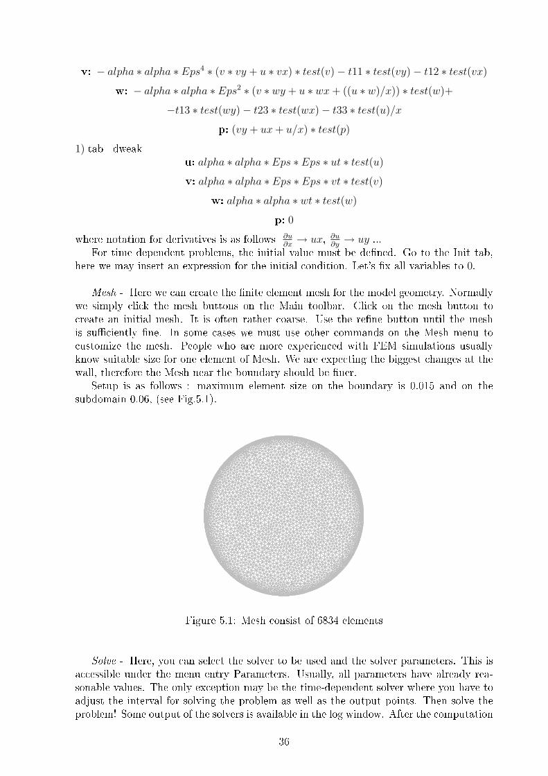
Mesh - Here we can create the nite element mesh for the model geometry. Normallywe simply click the mesh buttons on the Main toolbar. Click on the mesh button tocreate an initial mesh. It is often rather coarse. Use the rene button until the meshis suciently ne. In some cases we must use other commands on the Mesh menu tocustomize the mesh. People who are more experienced with FEM simulations usuallyknow suitable size for one element of Mesh. We are expecting the biggest changes at thewall, therefore the Mesh near the boundary should be ner.
Setup is as follows : maximum element size on the boundary is 0.015 and on thesubdomain 0.06, (see Fig.5.1).
Figure 5.1: Mesh consist of 6834 elements
Solve - Here, you can select the solver to be used and the solver parameters. This isaccessible under the menu entry Parameters. Usually, all parameters have already rea-sonable values. The only exception may be the time-dependent solver where you have toadjust the interval for solving the problem as well as the output points. Then solve theproblem! Some output of the solvers is available in the log window. After the computation
36
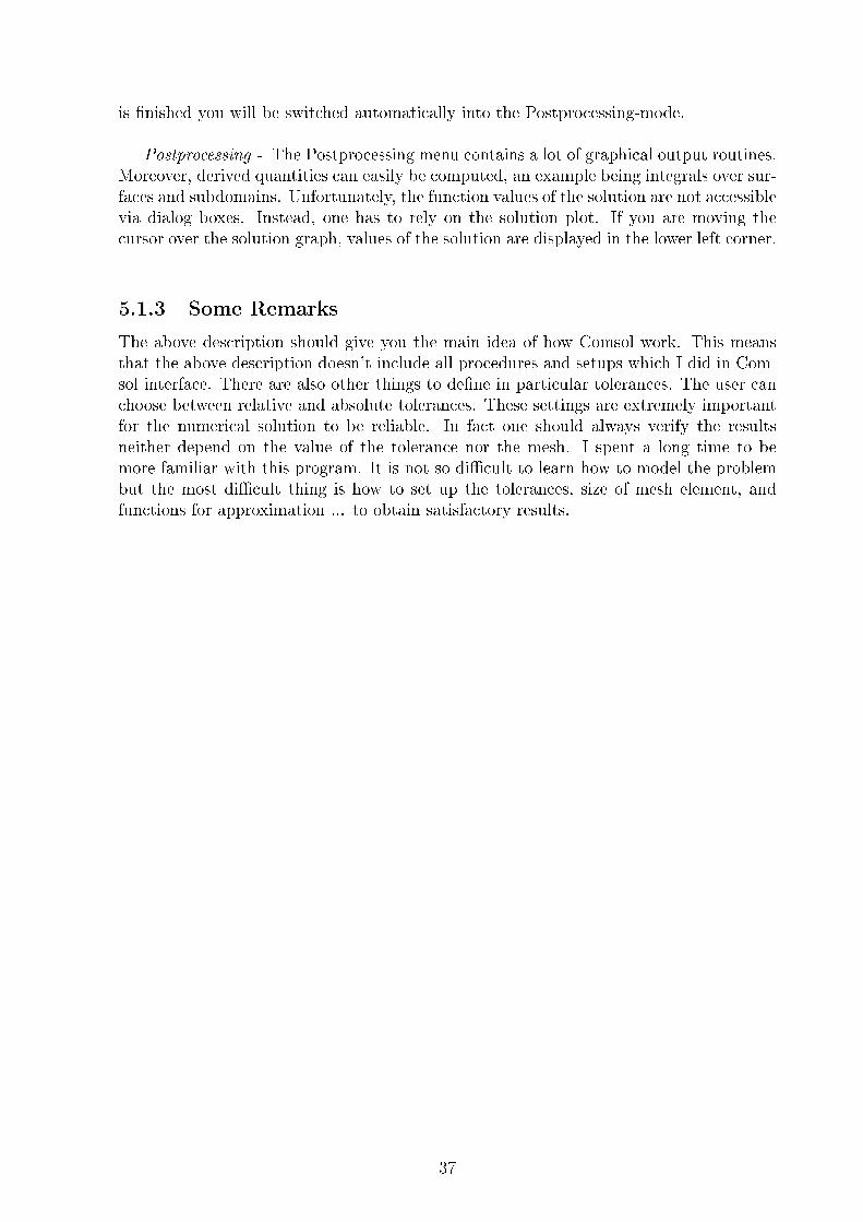
is nished you will be switched automatically into the Postprocessing-mode.
Postprocessing - The Postprocessing menu contains a lot of graphical output routines.Moreover, derived quantities can easily be computed, an example being integrals over sur-faces and subdomains. Unfortunately, the function values of the solution are not accessiblevia dialog boxes. Instead, one has to rely on the solution plot. If you are moving thecursor over the solution graph, values of the solution are displayed in the lower left corner.
5.1.3 Some Remarks
The above description should give you the main idea of how Comsol work. This meansthat the above description doesn't include all procedures and setups which I did in Com-sol interface. There are also other things to dene in particular tolerances. The user canchoose between relative and absolute tolerances. These settings are extremely importantfor the numerical solution to be reliable. In fact one should always verify the resultsneither depend on the value of the tolerance nor the mesh. I spent a long time to bemore familiar with this program. It is not so dicult to learn how to model the problembut the most dicult thing is how to set up the tolerances, size of mesh element, andfunctions for approximation ... to obtain satisfactory results.
37
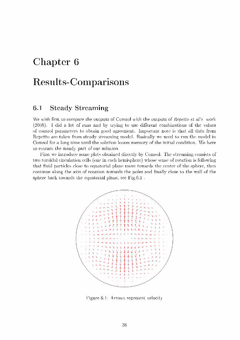
Chapter 6
Results-Comparisons
6.1 Steady Streaming
We wish rst to compare the outputs of Comsol with the outputs of Repetto et al's work(2008). I did a lot of runs and by trying to use dierent combinations of the valuesof control parameters to obtain good agreement. Important note is that all data fromRepetto are taken from steady streaming model. Basically we need to run the model inComsol for a long time until the solution looses memory of the initial condition. We haveto extract the steady part of our solution.
First we introduce some plots obtained directly by Comsol. The streaming consists oftwo toroidal circulation cells (one in each hemisphere) whose sense of rotation is followingthat uid particles close to equatorial plane move towards the center of the sphere, thencontinue along the axis of rotation towards the poles and nally close to the wall of thesphere back towards the equatorial plane, see Fig.6.1 .
Figure 6.1: Arrows represent velocity
38
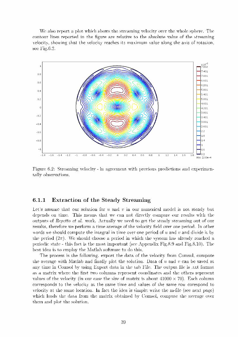
We also report a plot which shows the streaming velocity over the whole sphere. Thecontour lines reported in the gure are relative to the absolute value of the streamingvelocity, showing that the velocity reaches its maximum value along the axis of rotation,see Fig.6.2.
Figure 6.2: Streaming velocity - in agreement with previous predictions and experimen-tally observations.
6.1.1 Extraction of the Steady Streaming
Let's assume that our solution for u and v in our numerical model is not steady butdepends on time. This means that we can not directly compare our results with theoutputs of Repetto et al. work. Actually we need to get the steady streaming out of ourresults, therefore we perform a time average of the velocity eld over one period. In otherwords we should compute the integral in time over one period of u and v and divide it bythe period (2π). We should choose a period in which the system has already reached aperiodic state - this fact is the most important (see Appendix Fig.8.9 and Fig.8.10). Thebest idea is to employ the Matlab software to do this.
The process is the following, export the data of the velocity from Comsol, computethe average with Matlab and nally plot the solution. Data of u and v can be saved atany time in Comsol by using Export data in the tab File. The output le is .txt formatas a matrix where the rst two columns represent coordinates and the others representvalues of the velocity (in our case the size of matrix is about 41000 × 70). Each columncorresponds to the velocity at the same time and values of the same row corespond tovelocity at the same location. In fact the idea is simple: write the m-le (see next page)which loads the data from the matrix obtained by Comsol, compute the average overthem and plot the solution.
39
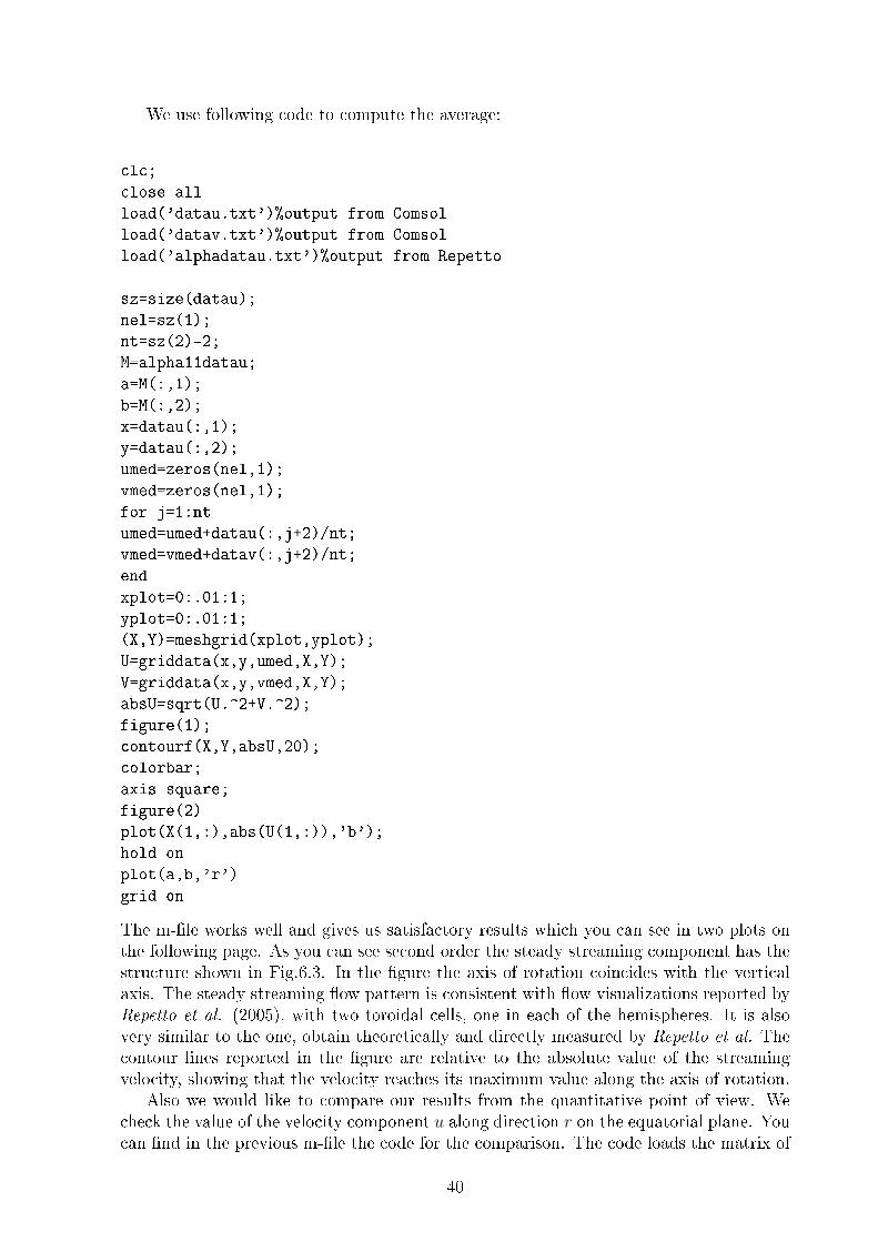
We use following code to compute the average:
clc;
close all
load('datau.txt')%output from Comsol
load('datav.txt')%output from Comsol
load('alphadatau.txt')%output from Repetto
sz=size(datau);
nel=sz(1);
nt=sz(2)-2;
M=alpha11datau;
a=M(:,1);
b=M(:,2);
x=datau(:,1);
y=datau(:,2);
umed=zeros(nel,1);
vmed=zeros(nel,1);
for j=1:nt
umed=umed+datau(:,j+2)/nt;
vmed=vmed+datav(:,j+2)/nt;
end
xplot=0:.01:1;
yplot=0:.01:1;
(X,Y)=meshgrid(xplot,yplot);
U=griddata(x,y,umed,X,Y);
V=griddata(x,y,vmed,X,Y);
absU=sqrt(U.^2+V.^2);
figure(1);
contourf(X,Y,absU,20);
colorbar;
axis square;
figure(2)
plot(X(1,:),abs(U(1,:)),'b');
hold on
plot(a,b,'r')
grid on
The m-le works well and gives us satisfactory results which you can see in two plots onthe following page. As you can see second order the steady streaming component has thestructure shown in Fig.6.3. In the gure the axis of rotation coincides with the verticalaxis. The steady streaming ow pattern is consistent with ow visualizations reported byRepetto et al. (2005), with two toroidal cells, one in each of the hemispheres. It is alsovery similar to the one, obtain theoretically and directly measured by Repetto et al. Thecontour lines reported in the gure are relative to the absolute value of the streamingvelocity, showing that the velocity reaches its maximum value along the axis of rotation.
Also we would like to compare our results from the quantitative point of view. Wecheck the value of the velocity component u along direction r on the equatorial plane. Youcan nd in the previous m-le the code for the comparison. The code loads the matrix of
40
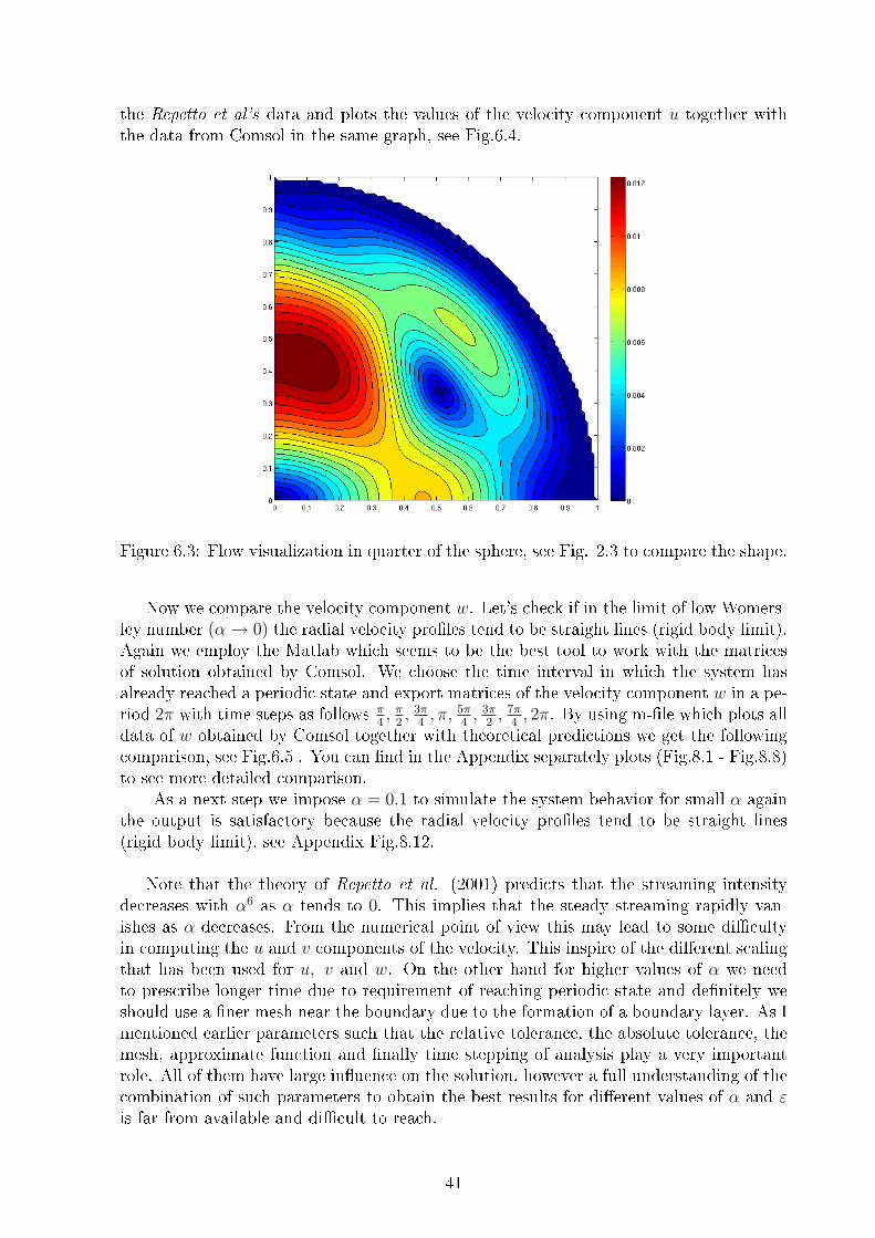
the Repetto et al's data and plots the values of the velocity component u together withthe data from Comsol in the same graph, see Fig.6.4.
Figure 6.3: Flow visualization in quarter of the sphere, see Fig. 2.3 to compare the shape.
Now we compare the velocity component w. Let's check if in the limit of low Womers-ley number (α→ 0) the radial velocity proles tend to be straight lines (rigid body limit).Again we employ the Matlab which seems to be the best tool to work with the matricesof solution obtained by Comsol. We choose the time interval in which the system hasalready reached a periodic state and export matrices of the velocity component w in a pe-riod 2π with time steps as follows π
4, π
2, 3π
4, π, 5π
4, 3π
2, 7π
4, 2π. By using m-le which plots all
data of w obtained by Comsol together with theoretical predictions we get the followingcomparison, see Fig.6.5 . You can nd in the Appendix separately plots (Fig.8.1 - Fig.8.8)to see more detailed comparison.
As a next step we impose α = 0.1 to simulate the system behavior for small α againthe output is satisfactory because the radial velocity proles tend to be straight lines(rigid body limit), see Appendix Fig.8.12.
Note that the theory of Repetto et al. (2001) predicts that the streaming intensitydecreases with α6 as α tends to 0. This implies that the steady streaming rapidly van-ishes as α decreases. From the numerical point of view this may lead to some dicultyin computing the u and v components of the velocity. This inspire of the dierent scalingthat has been used for u, v and w. On the other hand for higher values of α we needto prescribe longer time due to requirement of reaching periodic state and denitely weshould use a ner mesh near the boundary due to the formation of a boundary layer. As Imentioned earlier parameters such that the relative tolerance, the absolute tolerance, themesh, approximate function and nally time stepping of analysis play a very importantrole. All of them have large inuence on the solution, however a full understanding of thecombination of such parameters to obtain the best results for dierent values of α and εis far from available and dicult to reach.
41
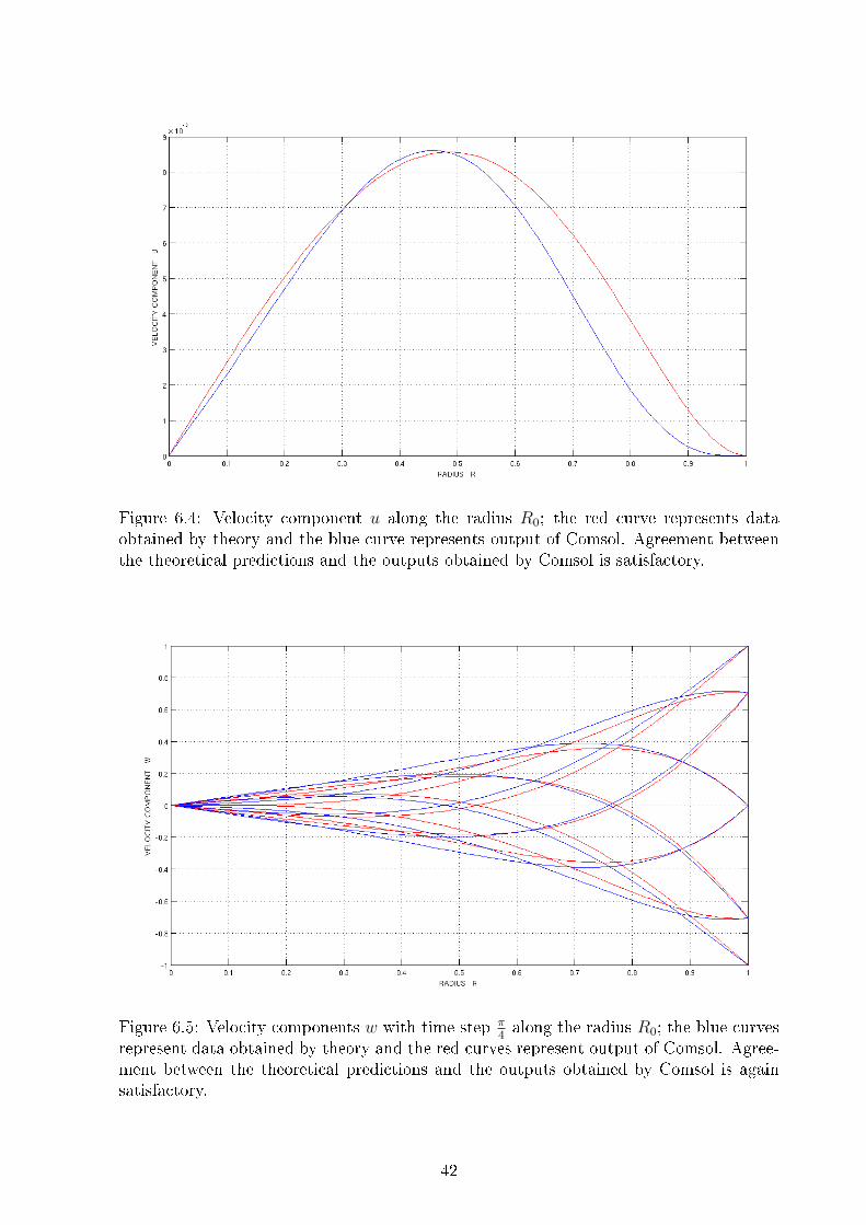
Figure 6.4: Velocity component u along the radius R0; the red curve represents dataobtained by theory and the blue curve represents output of Comsol. Agreement betweenthe theoretical predictions and the outputs obtained by Comsol is satisfactory.
Figure 6.5: Velocity components w with time step π4along the radius R0; the blue curves
represent data obtained by theory and the red curves represent output of Comsol. Agree-ment between the theoretical predictions and the outputs obtained by Comsol is againsatisfactory.
42
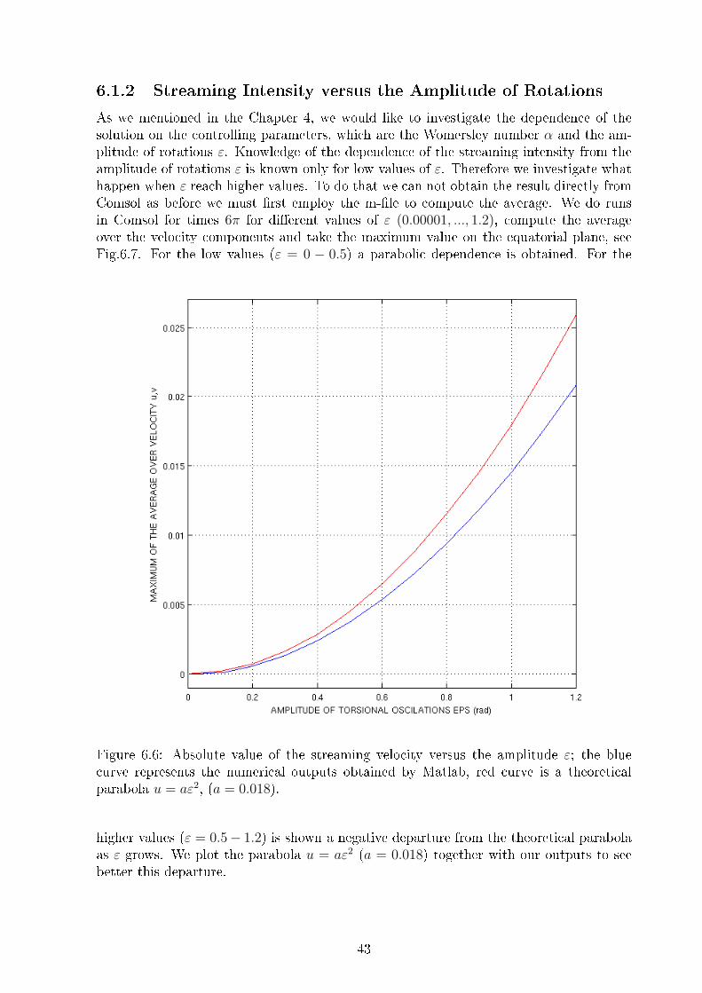
6.1.2 Streaming Intensity versus the Amplitude of Rotations
As we mentioned in the Chapter 4, we would like to investigate the dependence of thesolution on the controlling parameters, which are the Womersley number α and the am-plitude of rotations ε. Knowledge of the dependence of the streaming intensity from theamplitude of rotations ε is known only for low values of ε. Therefore we investigate whathappen when ε reach higher values. To do that we can not obtain the result directly fromComsol as before we must rst employ the m-le to compute the average. We do runsin Comsol for times 6π for dierent values of ε (0.00001, ..., 1.2), compute the averageover the velocity components and take the maximum value on the equatorial plane, seeFig.6.7. For the low values (ε = 0 − 0.5) a parabolic dependence is obtained. For the
Figure 6.6: Absolute value of the streaming velocity versus the amplitude ε; the bluecurve represents the numerical outputs obtained by Matlab, red curve is a theoreticalparabola u = aε2, (a = 0.018).
higher values (ε = 0.5− 1.2) is shown a negative departure from the theoretical parabolaas ε grows. We plot the parabola u = aε2 (a = 0.018) together with our outputs to seebetter this departure.
43
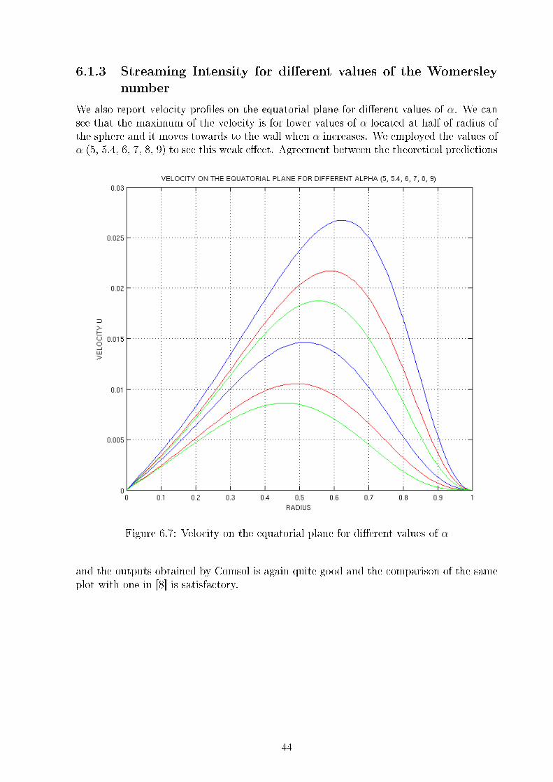
6.1.3 Streaming Intensity for dierent values of the Womersley
number
We also report velocity proles on the equatorial plane for dierent values of α. We cansee that the maximum of the velocity is for lower values of α located at half of radius ofthe sphere and it moves towards to the wall when α increases. We employed the values ofα (5, 5.4, 6, 7, 8, 9) to see this weak eect. Agreement between the theoretical predictions
Figure 6.7: Velocity on the equatorial plane for dierent values of α
and the outputs obtained by Comsol is again quite good and the comparison of the sameplot with one in [8] is satisfactory.
44
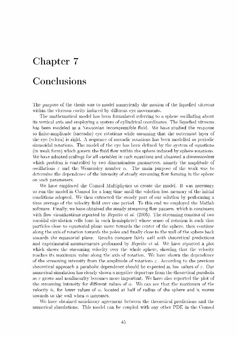
Chapter 7
Conclusions
The purpose of the thesis was to model numerically the motion of the liqueed vitreouswithin the vitreous cavity induced by dierent eye movements.
The mathematical model has been formulated referring to a sphere oscillating aboutits vertical axis and employing a system of cylindrical coordinates. The liqueed vitreoushas been modeled as a Newtonian incompressible uid. We have studied the responseto nite-amplitude (saccadic) eye rotations while assuming that the outermost layer ofthe eye (sclera) is rigid. A sequence of saccadic rotations has been modelled as periodicsinusoidal rotations. The model of the eye has been dened by the system of equations(in weak form) which govern the uid ow within the sphere induced by sphere rotations.We have adopted scalings for all variables in such equations and obtained a dimensionlesswhich problem is controlled by two dimensionless parameters, namely the amplitude ofoscillations ε and the Womersley number α. The main purpose of the work was todetermine the dependence of the intensity of steady streaming ow forming in the sphereon such parameters.
We have employed the Comsol Multiphysics to create the model. It was necessaryto run the model in Comsol for a long time until the solution lost memory of the initialconditions adopted. We then extracted the steady part of our solution by performing atime average of the velocity eld over one period. To this end we employed the Matlabsoftware. Finally, we have obtained the steady streaming ow pattern, which is consistentwith ow visualizations reported by Repetto et al. (2005). The streaming consists of twotoroidal circulation cells (one in each hemisphere) whose sense of rotation is such thatparticles close to equatorial plane move towards the center of the sphere, then continuealong the axis of rotation towards the poles and nally close to the wall of the sphere backtowards the equatorial plane. Results compare fairly well with theoretical predictionsand experimental measurements performed by Repetto et al. We have reported a plotwhich shows the streaming velocity over the whole sphere, showing that the velocityreaches its maximum value along the axis of rotation. We have shown the dependenceof the streaming intensity from the amplitude of rotations ε. According to the previoustheoretical approach a parabolic dependence should be expected at low values of ε. Ournumerical simulation has clearly shown a negative departure from the theoretical parabolaas ε grows and nonlinearity becomes more important. We have also reported the plot ofthe streaming intensity for dierent values of α. We can see that the maximum of thevelocity is, for lower values of α, located at half of radius of the sphere and it movestowards to the wall when α increases.
We have obtained satisfatory agreement between the theoretical predictions and thenumerical simulations. This model can be coupled with any other PDE in the Comsol
45

interface such as to an advection-diusion equation. This will allow to quantify the mixingprocesses within the vitreous cavity, which is of major clinical signicance to understandthe behaviour of drugs directly injected in the vitreous cavity.
46
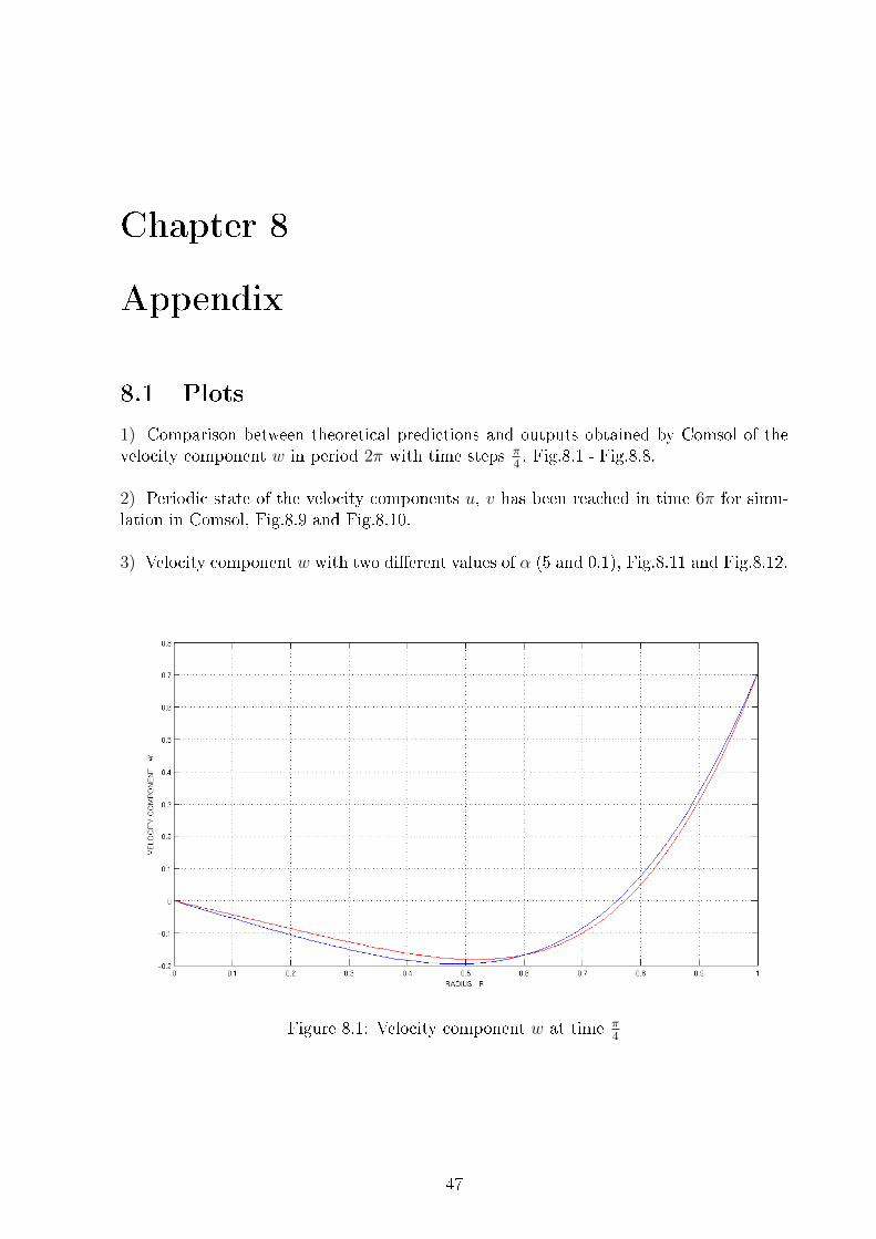
Chapter 8
Appendix
8.1 Plots
1) Comparison between theoretical predictions and outputs obtained by Comsol of thevelocity component w in period 2π with time steps π
4, Fig.8.1 - Fig.8.8.
2) Periodic state of the velocity components u, v has been reached in time 6π for simu-lation in Comsol, Fig.8.9 and Fig.8.10.
3) Velocity component w with two dierent values of α (5 and 0.1), Fig.8.11 and Fig.8.12.
Figure 8.1: Velocity component w at time π4
47
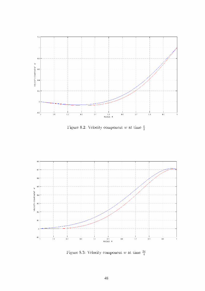
Figure 8.2: Velocity component w at time π2
Figure 8.3: Velocity component w at time 3π4
48
Figure 8.4: Velocity component w at time π
Figure 8.5: Velocity component w at time 5π4
49
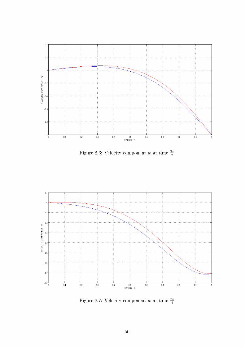
Figure 8.6: Velocity component w at time 3π2
Figure 8.7: Velocity component w at time 7π4
50
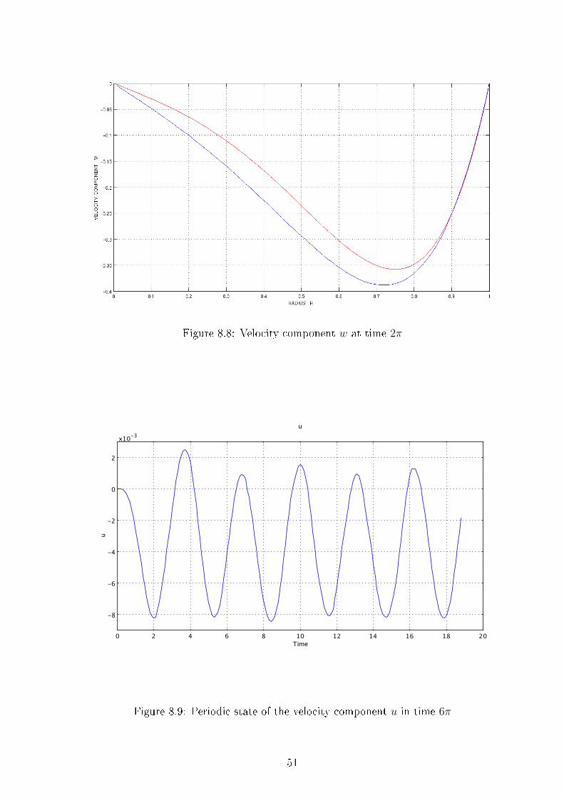
Figure 8.8: Velocity component w at time 2π
Figure 8.9: Periodic state of the velocity component u in time 6π
51
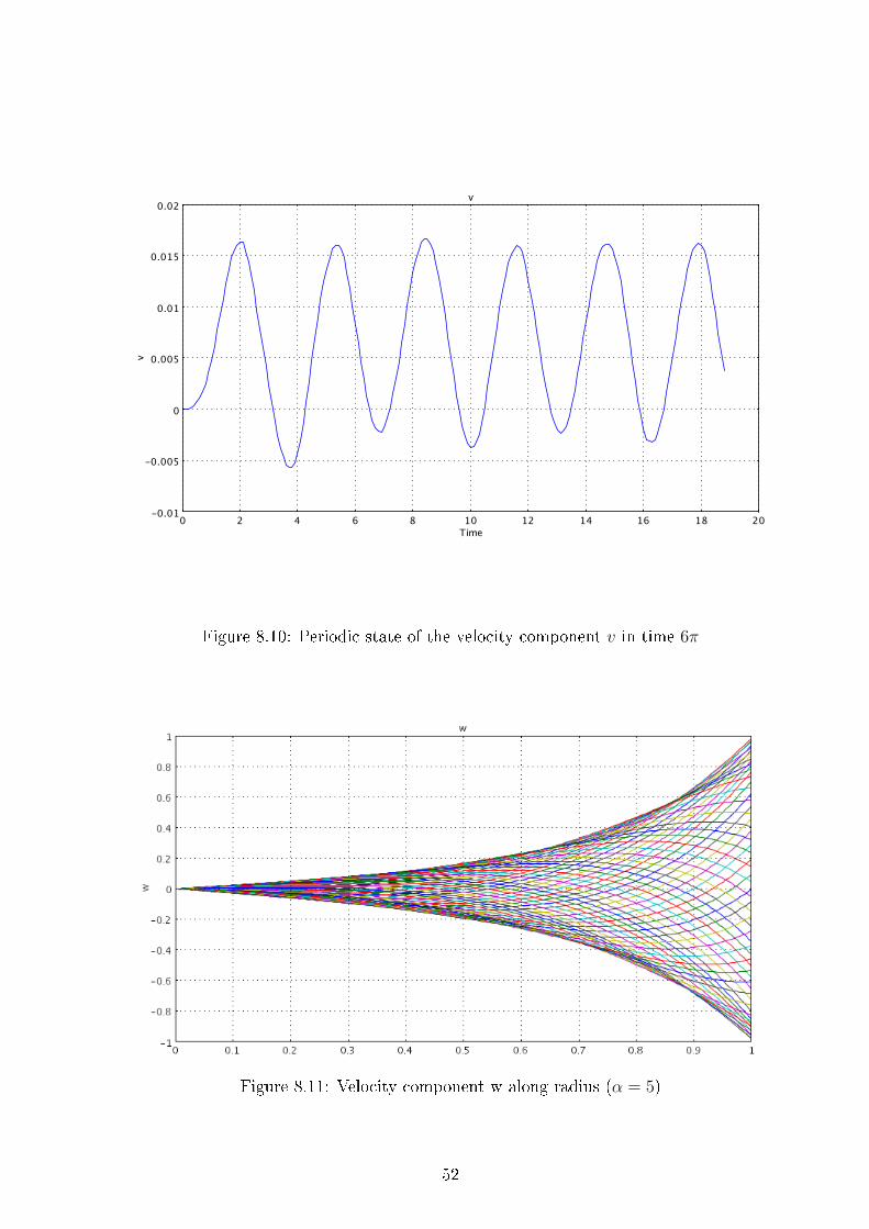
Figure 8.10: Periodic state of the velocity component v in time 6π
Figure 8.11: Velocity component w along radius (α = 5)
52
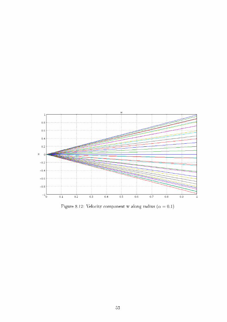
Figure 8.12: Velocity component w along radius (α = 0.1)
53
Bibliography
[1] David, T., Smye, S., Dabbs, T. and James, T., 1998, A model for the uid motion ofvitreous humour of the human eye during saccadic movements, Phys. Med. Biol. 43,pp. 1385-1399.
[2] Xu, J., Heys, J. J. and Barocas, V. H.. 2000. Permeability and diusion in vitreoushumor: implications for drug delivery, Pharmaceutical Research, 17, No. 6, pp. 664-669.
[3] Maurice, D. 2001. Review: practical issues in intravitreal drug delivery, Journal ofOcular Pharmacology, 17, No. 4, pp. 393-401.
[4] Stocchino, A., Repetto, R. and Caerata, C. 2007. Eye rotation induced dynamics ofa Newtonian uid within the vitreous cavity: the eect of the chamber shape, Phys.Med. Biol., 52, pp. 2021-2034.
[5] Repetto, R. 2006. An analytical model of the dynamics of the liqueed vitreous inducedby saccadic eye movements, Meccanica, 41, No. 1, pp 101-117.
[6] Caerata, C., Repetto, R., Siggers, J. and Stocchino, A. , June 2006. Fluid dynamicevents within the vitreous cavity induced by saccadic eye rotations. ASME 2007 Summer Bioengineering Conference, Keystone, CO, USA. June 20-24, 2007.
[7] Reddy, J. N. 2005. An Introduction to the Finite Element Method, Tata McGraw-HillEdition, Third Edition, pp. 19-57.
[8] Repetto, R. and Siggers, J. H. and Stocchino, A., 2008. Steady streaming within aperiodically rotating sphere, Journal of Fluid Mechanics, 608.
[9] H. Lund-Andersen, 2003. Adler's physiology of the eye. P. L. Kaufman and A. Alm,Mosby
[10] J. Sebag, 1989. The vitreous: Structure, Function and Pathobiology, Springer andVerlag.
[11] W. Becker, 1989. The neurobiology of saccadic eye movements, Elsevier Science Pub-lisher BV (Biomedical Division), R.H. Wurtz and M.E. Goldberg.
[12] Repetto, R. 2005. Experimental investigation of vitreous humour motion within ahuman eye model, Phys. Med. Biol. 50 (2005) 47294743.
[13] C. Loudon and A. Tordesillas, 1998. The use of the dimensionless Womersley numberto characterize the unsteady nature of internal ow, J. theor. Biol., 191., 63-78.
54


