Implementace algoritmu pro zpracov˚ an´ ´ı · cessing Element (PPE), which is a general-purpose...

UNIVERZITA KARLOVA V PRAZE

MATEMATICKO-FYZIKALNI FAKULTA

DIPLOMOVA PRACE

Bc. Vaclav Klecanda

Implementace algoritmu pro zpracovanıobrazu na IBM Cell

Kabinet software a vyuky informatikyVedoucı diplomove prace: Mgr. Vaclav Krajıcek

Studijnı program: Informatika, softwarove systemy

Rad bych podekoval magistru Vaclavu Krajıckovi za jeho vedenı, rady, nazory apripomınky a vubec za jeho podporu. Dale chci podekovat svym rodicum a meprıtelkyni za trpelivost.

I would like to thank to Mgr. Vaclav Krajıcek for leading, his advices, opinionsand other support. I also want to thank to my parents and to my girlfriend for theirpatience during works on this thesis.

Prohlasuji, ze jsem svou diplomovou praci napsal samostatne a vyhradne s pouzitımcitovanych pramenu. Souhlasım se zapujcovanım prace.

V Praze dne 4. Srpna 2009 Vaclav Klecandavlastnorucnı podpis

Contents

1 Introduction 9

2 Cell/B.E. platform 112.1 PPE - Power Processing Element . . . . . . . . . . . . . . . . . . . 132.2 SPE - Synergistic Processing Element . . . . . . . . . . . . . . . . 13

3 Cell/B.E. programming 153.1 Cell/B.E. platform development . . . . . . . . . . . . . . . . . . . 153.2 SDK content . . . . . . . . . . . . . . . . . . . . . . . . . . . . . . 163.3 Parallel systems & Cell/B.E. . . . . . . . . . . . . . . . . . . . . . 173.4 Cell/B.E. programming models . . . . . . . . . . . . . . . . . . . . 18

3.4.1 Cell/B.E. parallelism levels . . . . . . . . . . . . . . . . . . 193.4.2 Computation configurations . . . . . . . . . . . . . . . . . 20

3.5 Building for the Cell/B.E. . . . . . . . . . . . . . . . . . . . . . . . 223.5.1 Process of application porting for the Cell/B.E. . . . . . . . 223.5.2 SPE porting considerations . . . . . . . . . . . . . . . . . . 253.5.3 Speed and compiler options . . . . . . . . . . . . . . . . . 26

3.6 Profiling . . . . . . . . . . . . . . . . . . . . . . . . . . . . . . . . 27

4 Image segmentation 284.1 Problem formulation . . . . . . . . . . . . . . . . . . . . . . . . . 284.2 Image segmentation methods overview . . . . . . . . . . . . . . . . 294.3 Level set . . . . . . . . . . . . . . . . . . . . . . . . . . . . . . . . 31

4.3.1 Level set theory . . . . . . . . . . . . . . . . . . . . . . . . 324.3.2 Level set computation . . . . . . . . . . . . . . . . . . . . 324.3.3 Speed-up approaches . . . . . . . . . . . . . . . . . . . . . 334.3.4 Level set image segmentation . . . . . . . . . . . . . . . . 364.3.5 Level set methods on streaming architectures . . . . . . . . 38

5 Design and implementation 405.1 Original idea of the porting process . . . . . . . . . . . . . . . . . . 405.2 Chosen algorithm and frameworks . . . . . . . . . . . . . . . . . . 415.3 Incorporation into MedV4D framework . . . . . . . . . . . . . . . 41

5.3.1 Client part . . . . . . . . . . . . . . . . . . . . . . . . . . 435.3.2 Server part . . . . . . . . . . . . . . . . . . . . . . . . . . 45

3

5.4 Level set segmentation pipeline . . . . . . . . . . . . . . . . . . . . 465.5 Pre-porting steps . . . . . . . . . . . . . . . . . . . . . . . . . . . 475.6 Profiling . . . . . . . . . . . . . . . . . . . . . . . . . . . . . . . . 495.7 New design . . . . . . . . . . . . . . . . . . . . . . . . . . . . . . 50

5.7.1 Data flow . . . . . . . . . . . . . . . . . . . . . . . . . . . 515.7.2 Tools . . . . . . . . . . . . . . . . . . . . . . . . . . . . . 525.7.3 Work balancing . . . . . . . . . . . . . . . . . . . . . . . . 54

5.8 Actual porting process . . . . . . . . . . . . . . . . . . . . . . . . 545.8.1 PC as Cell/B.E. simulator . . . . . . . . . . . . . . . . . . 545.8.2 Moving to PPE . . . . . . . . . . . . . . . . . . . . . . . . 555.8.3 Tools porting . . . . . . . . . . . . . . . . . . . . . . . . . 555.8.4 Memory checking tools . . . . . . . . . . . . . . . . . . . . 55

6 Results 576.1 Speed measurements . . . . . . . . . . . . . . . . . . . . . . . . . 576.2 Reasons of slowdown and possible improvements . . . . . . . . . . 586.3 Code and design complexity . . . . . . . . . . . . . . . . . . . . . 61

7 Conclusion 63

A Images 67

B Tools setup 72B.1 SDK installation . . . . . . . . . . . . . . . . . . . . . . . . . . . . 72

B.1.1 Bug fixing . . . . . . . . . . . . . . . . . . . . . . . . . . 74B.2 IBM Full-System Simulator . . . . . . . . . . . . . . . . . . . . . 74

B.2.1 Bug fixing . . . . . . . . . . . . . . . . . . . . . . . . . . 75B.2.2 Installation of libraries into sysroot image . . . . . . . . . . 77B.2.3 Copying content into sysroot image . . . . . . . . . . . . . 77B.2.4 Simulator hints . . . . . . . . . . . . . . . . . . . . . . . . 77

B.3 Using examples . . . . . . . . . . . . . . . . . . . . . . . . . . . . 78B.4 Tuning memory usage on PS3 . . . . . . . . . . . . . . . . . . . . 78B.5 Performance tools . . . . . . . . . . . . . . . . . . . . . . . . . . . 79B.6 Visual Performance Analyser - VPA . . . . . . . . . . . . . . . . . 79B.7 Cell/B.E. cross compilation . . . . . . . . . . . . . . . . . . . . . . 79

C Content of the DVD 80

List of Figures

2.1 Cell/B.E. processor layout . . . . . . . . . . . . . . . . . . . . . . 122.2 Cell/B.E. based machines . . . . . . . . . . . . . . . . . . . . . . . 14

3.1 Streaming SPE configuration . . . . . . . . . . . . . . . . . . . . . 203.2 Pipeline SPE configuration . . . . . . . . . . . . . . . . . . . . . . 213.3 PPE centric configuration . . . . . . . . . . . . . . . . . . . . . . . 213.4 SPE binary embedding . . . . . . . . . . . . . . . . . . . . . . . . 233.5 Application porting cycle . . . . . . . . . . . . . . . . . . . . . . . 25

4.1 Flooding an object . . . . . . . . . . . . . . . . . . . . . . . . . . 314.2 Narrow band computation illustration . . . . . . . . . . . . . . . . 334.3 Sparse fields method computation illustration . . . . . . . . . . . . 354.4 Graph of thresholding based speed function . . . . . . . . . . . . . 374.5 Leaking . . . . . . . . . . . . . . . . . . . . . . . . . . . . . . . . 374.6 GPU virtual memory . . . . . . . . . . . . . . . . . . . . . . . . . 39

5.1 LevelSetClient application computation process . . . . . . . . . . . 425.2 ITK wrapper MedV4D filter . . . . . . . . . . . . . . . . . . . . . 435.3 Remote MedV4D filter . . . . . . . . . . . . . . . . . . . . . . . . 445.4 MedV4D server cycle . . . . . . . . . . . . . . . . . . . . . . . . . 455.5 Original ITK thresholding level set filter class hierarchy . . . . . . . 485.6 Resulting level set filter ready to be ported to Cell/B.E. . . . . . . . 495.7 Diagram of new design components . . . . . . . . . . . . . . . . . 50

6.1 Automatic align of small data . . . . . . . . . . . . . . . . . . . . . 596.2 Multiple DMA list workaround . . . . . . . . . . . . . . . . . . . . 596.3 Comparison of one slice segmented on different architectures . . . . 60

A.1 3D view of segmented skull data set . . . . . . . . . . . . . . . . . 67A.2 Result of segmentation of parietal part of a skull . . . . . . . . . . . 68A.3 Result of segmentation middle slices of the skull data set . . . . . . 69A.4 Result of segmentation front slices of the skull data set . . . . . . . 70A.5 Result of segmentation of slices near nose . . . . . . . . . . . . . . 71A.6 3d blending of original and segmentationed images . . . . . . . . . 71

B.1 Screenshot of standard cellide veiw . . . . . . . . . . . . . . . . . 75B.2 Cellide with started simulator . . . . . . . . . . . . . . . . . . . . . 76

5

List of Tables

5.1 Profiling results . . . . . . . . . . . . . . . . . . . . . . . . . . . . 49

6.1 Measurement results . . . . . . . . . . . . . . . . . . . . . . . . . 58

6

Nazev prace: Implementace algoritmu pro zpracovanı obrazu na IBM CellAutor: Bc. Vaclav KlecandaKatedra (ustav): Kabinet software a vyuky informatikyVedoucı diplomove prace: Mgr. Vaclav Krajıceke-mail vedoucıho: [email protected]:

Prace shrnuje dostupne informace o architekture IBM Cell/B.E. tak, aby ctenarrychle zıskal potrebny nahled na problematiku programovanı pro tuto architekturu.Prakticke informace jsou cerpany z vyvoje aplikace ktera implementuje netrivialnıalgoritmus z oblasti zpracovanı obrazu, sparse field level set segmentation. Dalsıcast obsahuje popis vyvoje teto aplikace a resenı problemu, ktere mohou behemnej nastat.

Prace zaroven srovnava klasickou a Cell architekturu a popisuje nutne podmınkypro vytvorenı efektivnı aplikace pro Cell/B.E. Dale obsahuje strucny postupinstalace nejdulezitejsıch vyvojovych nastroju. Tento postup si klade za cıl conejrychleji pripravit vse potrebne a zkratit tak dobu prıpravne faze tak, aby ctenarmohl zacıt vyvıjet pro Cell/B.E.

Klıcova slova: programovanı pro Cell, multicore acceleration, IBM, PS3

Title: Implementation of image processing algorithms on IBM CellAuthor: Bc. Vaclav KlecandaDepartment: Department of Software and Computer Science EducationSupervisor: Mgr. Vaclav KrajıcekSupervisor’s e-mail address: [email protected]:

This work summarize available information about IBM Cell/B.E. architecture tolet the reader create a necessary overview for programming for this architecture.Practical information are based on development of an application that implementsnontrivial image processing algorithm, sparse field level set segmentation. Nextsection contains description of the application development and associatedproblems solving.

The work compares common and Cell B.E. architectures and describes conditionsnecessary for creation of an effective Cell/B.E. application. The work alsocontains brief procedure of the most important development tools installation.This procedure has to prepare everything necessary as fast as possible and thus toshorten the duration of the preparation phase to let the reader to start development.

Keywords: CellBE programming, multi-core acceleration, IBM, PS3

Chapter 1

Introduction

The production of x86 platform processors has started a big frequency competition.The manufacturers have been releasing processors with higher and higher operat-ing frequency. Behind this competition there has been a significant amount of re-search of new production technologies that allow to integrate more transistors ontoa smaller area. Gradually the manufacturers started to realize that it is impossibleto continue the competition forever.

More computing units started to be integrated into a single processor. The firstamong common desktop processors was Intel’s Pentium R© with hyper-threading.This processor was able to execute two threads at a time. Since then a quick boomof multi-core integration started even among other big processor manufacturers.

Integration of more execution cores allows less power consumption. This factoris nowadays especially important due to processor integration into laptops and evendue to environmental issues. Therefore current effort of the processor manufactur-ers is to gain the best performance to power consumption ratio.

General purpose cores are integrated into the current common processors.It means they have a pipeline for instruction execution composed of severalstages. Instruction can be in various states in the pipeline, e.g. fetched, awaitingoperands, ready, executed. Instructions do not flow among the stages in the orderthat designates the program but the order is decided by the processor itself. Thedecision is based on variety of factors and predictions. One of the pipeline stagesis a branch-prediction unit. It has to predict the most probable flow of the executedprogram. When this prediction is false the whole pipeline has to be discarded andexecution of the right branch of the program has to be started. Processors sufferheavily from these mispredictions because they lead into big execution holes inwhich the processor pipeline stalls or is being reset.

9

CHAPTER 1. INTRODUCTION 10

Cache misses are another general purpose processor suffering. A cache missoccurs when the requested data are not within processor cache and have to be loadedfrom the main memory.

Although many improvements were implemented into the general purpose pro-cessors they still suffer from the described problems. This is one of the reasons whya collaboration of three big companies IBM, Sony, and Toshiba started developmentof the Cell/B.E. processor. It is a multi-core processor which has high performanceto power consumption ratio and is able to overcome the problems that the generalpurpose processors suffer from. That is because it allows the programmer to man-age processor cache and branch prediction unit to a certain degree. The next chapterwill describe the processor in more details.

Chapter 2

Cell/B.E. platform

This chapter will introduce the Cell Broadband Engine processor (Cell/B.E.), thewhole platform and its specific details. The particular Cell/B.E. processor will bedescribed and illustrated. All the information were taken from [6].

Cell/B.E. processor is representative of a new generation of IBM’s Cell/B.E.platform family. Cell/B.E. is an asymmetric, high-performance multi-core proces-sor that combines eight synergistic processing elements (SPE) and a Power Pro-cessing Element (PPE), which is a general-purpose IBM Power PC R© core. Thenext important part is a central memory element. The PPE can operate with thecentral memory directly while the SPE can access the memory indirectly throughDMA. All the elements are connected through a high speed bus (EIB - ElementInterconnect Bus). The whole layout is in the figure 2.1.

The Cell/B.E. achieves a significantly better performance per Watt and perfor-mance per chip area ratios than conventional high-performance processors. It ismore flexible and programmable than single-function and other optimized proces-sors such as graphics processors, or conventional digital signal processors. Whilea conventional microprocessor may deliver about 20+GFlops of single-precision(32b) floating-point performance, Cell delivers 200+ GFlops (under ideal condi-tions) at a comparable power consumption.

A number of signal processing and media applications have been implementedon the Cell/B.E. with excellent results. Advanced visualization techniques suchas ray-casting, ray-tracing and volume rendering, streaming applications such asmedia encoders, decoders or encryption and decryption algorithms have also beendemonstrated to perform about an order of magnitude better than a conventionalprocessors.

11

CHAPTER 2. CELL/B.E. PLATFORM 12

PPE

EIB (High speed bus)

SystemMemory

...

SPE 0

local store

256 kB

128 128−bitregisters

SPU

core

DMA engine

SPE 7

local store

256 kB

128 128−bitregisters

SPU

core

DMA engine

Figure 2.1: One PPE unit along with eight SPE stream processor units and systemmemory connected together with a high speed EIB bus


2.1 PPE - Power Processing Element

The PPE is derived from IBM Power PC R© core. It has 512kB L2 on die cache. Itsupports the Power Architecture ISA, inherits the memory translation, protection,and SMP coherence model of mainstream 64-bit Power processors. Virtualization,logical partitioning, large pages, and other recent innovations in the Power architec-ture are supported as well. Programming for the PPE is the same as for conventionalprocessors due to direct access to central memory.

2.2 SPE - Synergistic Processing Element

SPE is an autonomous processor (sometimes called accelerator) targeted for com-putational intensive applications. Each SPE has a SIMD core (SPU), a high-speedprivate local store memory and a direct memory access (DMA) engine.

The SPU unit has 128 128-bit wide unified general purpose registers to storeall types of data in contrast to traditional RISC processors where registers are di-vided according data types. It supports a SIMD-RISC instruction set. The SPUhas two pipelines, the odd one and the even one, so it can execute two instructionsat a time (dual-issue) if some conditions are met. Vectorized operations in variousdata types configurations can be performed with these registers e.g. two double-precision floats or eight 32bit integers can be processed at single clock tick.

Unlike conventional microprocessors the SPE does not have a hardware cache.Its function represents the small on-chip local store memory under programmer’scontrol. This allows code optimizations that can reduce cache misses. The localstore is separated from the main memory i.e. the SPE has its own address space.Therefore any synchronization with other cores is not necessary. The SPE uses thelocal store as a cache of data stored in the central memory i.e. programmer has tocreate copies of the data within the local store. The data are transferred throughDMA engine which manages transferring data from central memory to local storeand vice versa as well as between two SPEs’ local stores. We say that data is”DMAed” from source to destination. DMA commands can be issued in manyways such as in synchronous, asynchronous or in scatter-gather manner throughDMA lists. The DMA list is an array of pointer-size pairs that defines pieces ofmemory that shall be transferred within single DMA request. The pieces must notnecessarily be continuous. Therefore the Cell/B.E. processor can be viewed as adistributed memory multiprocessor. The local store memory management is a bigpart of programming for the Cell/B.E.

Programming for the SPE is a bit different compared to programming for aconventional processor. Programmer have always to count with the fact that he/she


Figure 2.2: Images of Cell/B.E. based machines. Sony’s Play Station 3, on the left(image taken from www.boygeniusreport.com), IBM Cell Blade board, on the right(image taken from www.ps3tester.com)

has only 256kB for the program and data. More details about this topic will bedescribed in the next chapter.

The Cell/B.E. is embedded in game console Sony PlayStation 3 (PS3) as well asIBM Blade servers where are two processors on one board, building block. Therecan be more boards connected in one system forming a powerful and modular ma-chine. We have two PS3 machines available for this work.

Chapter 3

Cell/B.E. programming

Cell/B.E. platform development tools will be described in this chapter. Our expe-rience with the tools will be mentioned as well. Then particular SDK content andtools will be listed. Parallel systems and models will be mentioned later on as wellas the relationship to the Cell/B.E. development along with a few design patterns.At the end core configurations and their advantages and disadvantages will be listedfinishing with few practical approaches to the Cell/B.E. porting process.

3.1 Cell/B.E. platform development

IBM delivers a SDK for the Cell/B.E. application development. It is made for aLinux platform, in the concrete for the Fedora or the Red Hat distribution. It comesin two flavours. The first is the official non free SDK which has all the featuresneeded for the Cell/B.E. development even for hybrid systems. The purchaser hasalso a support team ready to help. The next is a free one that is open to wide publicand everybody can download it and start developing. The free one does not havefull support for hybrid systems nor for development in other languages than C/C++.We have used the free one since we have developed only in C/C++ and for a cleanCell/B.E. processor.

Because the SDK is for Linux operation system its user has to have alreadya deeper knowledge about this system. There are a few bugs and parts that arenot fully finished (see Appendix B) and without the deeper system knowledge ispractically impossible to react on an unexpected behaviour during installation ordevelopment phase.

We have begun with SDK version 3.0 and Fedora version 8 which were thecurrent versions of needed tools. We have faced a number of obstacles and beforewe were able to overcome them a new version of SDK (3.1) appeared. Because we

15

CHAPTER 3. CELL/B.E. PROGRAMMING 16

wanted to use and describe the latest tools we had to begin from scratch because thenew version brought new obstacles as well.

The new version was declared to be compatible with a new version of Fedora, 9- Sulphur, that had been released at almost the same time as the new SDK version.The previous version of SDK (3.0) was for Fedora 7 Werewolf. We have triedall possible combinations of Fedora distributions and SDK packages to find out ifthey are compatible with each other. The only result from that testings was findingout that they are not mutually compatible. We have spent plenty of days on thisdiscovery. The SDK is a huge package of software dependent on lots of third partylibraries and solutions. They are treated differently within particular distributionsand sometimes even versions of the same distribution. The resulting advise is toavoid combination of system versions nor SDK versions nor particular libraries thatthe SDK components are dependent on. The repository versions of the third partysoftware should be used.

Although there are too much of troubles when different version are combined,a few efforts to get the SDK run on another distributions than Fedora were made.But we think the time spent on this goal is not worth the result.

Finally we installed Fedora 9 Sulphur and SDK 3.1. Although this combinationis declared by IBM as tested we have run into few bugs and errors. The process ofinstallation is described in the Appendix B.

3.2 SDK content

The Cell/B.E. SDK is divided into variety of components. Each component is con-tained in one or more rpm package for easy installation purposes. Here is a list ofimportant available components:

1. Tool chain

Is a set of tools such as compilers, linkers etc. necessary for actual codegeneration. There are two tool chains. One is for PPU and the other for SPU.

2. Libraries

IBM provides several useful libraries for mathematical purposes e.g. linearalgebra, FFT, Monte Carlo with the SDK. Another libraries set is forcryptography or SPE run-time management. Code of these libraries isdebugged, highly optimized for running on SPEs and SIMDized. It is highlyadvisible to use the libraries i.e. adapt a code for using the libraries insteadof programming own solution.


3. Full system simulator

Program that can simulate the Cell/B.E. processor on other hardware plat-forms. It is used mostly in profiling stage because simulator can simulate ac-tual computation of a code in cycle precision. It can be of course used whenprogrammer has an actual Cell/B.E. hardware available, but the simulation isincredibly slow.

4. IDE

IDE is in fact version 3.2 of Eclipse with integration of debugging, profiling,Cell/B.E. machine management and other features that makes developmentfor the Cell/B.E. easier and more comfortable.

3.3 Parallel systems & Cell/B.E.

Parallelism depends on type of system where the program will be run. There aretwo basic kind of parallel systems:

1. shared-memory system

Is a multi-processor system with one shared memory which all processor cansee. Processors has to synchronize access to the memory otherwise race con-ditions will rise.

2. distributed-memory system

Is system where each processor has its own private memory. There is no needfor any synchronization.

In context of parallel systems Cell/B.E. is a kind of hybrid system. The SPEsmatches a distributed-memory system due to private local stores while the PPE isa shared-memory system. The Cell/B.E. is sometimes called heterogeneous multi-core processor with distributed memory. Because Cell/B.E. processors can be com-posed into bigger units such as IBM blade server with two Cell/B.E. chips they canbe viewed as either 16 + 2 cores in SMP mode or two non-uniform memory accessmachines connected together. Programmer has then to decide which view of theCell/B.E. processor is better for the solved problem.

Because of separation of address spaces programming of the SPE is very similarto client/server application design. Roles depends on how the work is started. Incase the PPU initiates the transfers, the PPU is a client and the SPE is a server be-cause the SPE receive data for computation and offer a service for the PPE. Anotherpossibility is that the SPE grabs the data from the central memory. In this case theSPE is a client of central memory. This scenario is preferred because the PPE isonly one and would not be able to manage all the SPUs.


3.4 Cell/B.E. programming models

Implementation of parallel algorithms rely on a parallel programming model. It isa set of software technologies such as programming languages extension, specialcompilers, libraries through that actual parallelism is achieved. The programmingmodel is programmer’s view to the hardware. Choosing a programming model ormixture of models that will best fit for the solved problem is another decision thatprogrammer has to make.

For the Cell/B.E. there is variety of parallel programming models. THe mod-els differ in view of the hardware from each other and thus how many actions areperformed implicitly by the model. The actions can be e.g. task distribution man-agement, data distribution management or synchronization. The most abstract onescan perform many actions implicitly. Their advantage is ease of implementationbut at cost no performance tuning ability. Differently act the most concrete modelsthat see the Cell/B.E. processor with all the low level details. Their advantage isperformance tuning ability in all application parts but at cost of more development.

There are several models that are targeted only for the Cell/B.E. platform andare contained in the SDK. While there are other models such as MPI, OpenMP thatcan be used as well but they would expose only the PPE. These will not be furtherdescribed.

List of the programming models (frameworks) follows in order from the mostconcrete to the most abstract:

1. libspe2

This library provides the most low level functionality. It offers SPE contextcreating, running, scheduling or deleting. DMA primitives for data transfer,mailboxes, signal, events, and synchronization functions for PPE to SPE andSPE to SPE dialogues are also provided by this library. More information canbe found in [7] within ”SPE Runtime Management Library” document.

2. Data Communication and Synchronization - DaCS

Defines a program entity for the PPE or the SPE. It is a HE (Host Elementprogram) for the PPE and an AE (Accelerator Element program) for theSPE. It provides variety of services for that programs. The services aree.g. resource and process management where an HE manipulates its AEs orgroup management, for defining groups in which synchronization events likebarriers can happen or message passing by using send and receive primitives.More information can be found in [7] within ”DACS Programmer’s Guideand API Reference” document.


3. Accelerated Library Framework - ALF

The ALF defines an ALF-task as another entity that perform computationallyintensive parts of a program. The idea is to have a program split into mul-tiple independent pieces which are called work blocks. They are describedby a computational kernel, the input and the output data. Programming withthe ALF is divided into two sides. The host and the accelerator one. On theaccelerator side the programmer has only to code the computational kernel,unwrap the input data, and pack the output data when the kernel finishes. TheALF offers clear separation between the host and the accelerator sides of pro-gram parts. It provides following services: work blocks queue management,load balancing between accelerators, transparent DMA transfers etc. Moreinformation can be found in [7] within ”ALF Programmer’s Guide and APIReference” document.

Choosing a framework is important decision of writing Cell/B.E. application. Itshould be considered enough.

3.4.1 Cell/B.E. parallelism levels

The Cell/B.E. processor offers four levels of parallel processing. That is because itis composed of heterogeneous elements, the SPE and the PPE and the possibility ofcomposition into a more complex systems. The levels are:

1. Server level

Parallelism on this level means task distribution among multiple servers likewithin a server farm. This is possible in a hybrid environment at the clusterlevel using MPI or some other grid computing middle-ware.

2. Cell/B.E. chips level

On this level tasks can be divided among multiple Cell/B.E. processors. Thisis possible if there are more such processors in single machine. It is e.g. IBMBlade server with two Cell/B.E. chips. ALF or DaCS for hybrid can be usedfor task distribution.

3. SPE level

This parallelism level allows to distribute tasks among particular SPEs. Lib-spe, ALF, DaCS can be used to perform the distribution.

4. SIMD instruction level

This level can increase the speed the most. Parallelism is achieved on instruc-tion level that means more data are processed at a time by single instruction.Language intrinsics are used for this purpose. This will be explained later inpart devoted to ”SIMDation”.


data source

SPE 2

SPE 0

SPE 3

SPE 1

data destination

Figure 3.1: All SPE run the same code creating farm of processor that process sametype of data.

3.4.2 Computation configurations

Because of the Cell/B.E.’s heterogeneous nature there are few computation config-urations that can be used. Each of them differs in usage of SPEs:

1. Streaming configuration

All SPEs serves as a stream processor (see figure 3.1). They run exactlythe same code expecting the same type of data and producing also the sameof data type. This configuration is well suited for streaming application forexample filters where there is still the same type of data on input.

2. Pipeline configuration

The SPEs are stages of a pipeline (see figure 3.2). Data are passed throughone SPE to another. This configuration makes use of the fact that transferamong SPEs is faster than the transfer between SPE and PPE.

3. PPE centric

This configuration is common approach to use the Cell/B.E. A program runson the PPE (see figure 3.3) and only selected, highly computational intensiveparts (hotspots) are offloaded to SPEs. This method is the easiest from aprogram development perspective because it limits the scope of source codechanges and does not require much re-engineering at the application logiclevel. A disadvantage is frequent changes of SPE contexts that is quiteexpensive operation.


PPE

SPE 3SPE 0 SPE 2SPE 1

PPE sends data to pipeline

last pipeline SPE sends result back to PPE

Figure 3.2: SPE creates a pipeline. Each SPE represent one stage of that pipeline.Data are transferred only via SPE to SPE DMA transfers benefiting the speed ofbus.

PPE runs program

hotspot is reached

SPE 0

SPE 1

SPE 2

program continues

hotspot

computation

management

Figure 3.3: Program is run on PPE and only hotspots are offloaded to SPEs. Of-floading means managing SPE context creation and loading as well as managingdata transfer and synchronization between PPE and SPEs


4. SPE server

Another configuration is to have server-like programs running on SPEs thatsits and waits offering specific services. It is very similar to the PPE centricconfiguration. Only difference is requirement to the program to be smallenough to fit into the SPU local store to avoid the frequent SPE contextswitching.

3.5 Building for the Cell/B.E.

Actual compilation process is performed using an appropriate tool chain. The PPEcode requires the PPE tool chain and the SPE code requires the SPE one. But thereis a difference between management of the code in linking stage between the PPEand the SPE object files. It is caused by difference of actual code usage. Whilethe PPU code resides in the central memory, like in common architectures, the SPUcode is loaded into the SPE dynamically and shall be somehow separated from thePPE code. It is similar to shader programs for graphic accelerators. They are alsoloaded into appropriate processors as soon as they are needed so they live separated.

There are two options for SPE code management. One is to build a shared li-brary and load it explicitly when it shall be used. Another way is to build a static li-brary and include it into the PPU executable using Cell/B.E. Embedded SPE ObjectFormat (CESOF). This allows PPE executable objects to contain SPE executablei.e. the SPE binary is embedded within the PPE binary, see figure 3.4. The SPUprogram is then referenced as special external structure directly from the PPU codeinstead of performing shared library loading. Both ways have advantages and disad-vantages which are the same as shared vs. static library usage. Shared library meansbetter modularity and possibility of code alternation without whole executable re-building. On the other hand additional management of such library is necessary incontrast to a static SPE code into a PPE binary embedding.

3.5.1 Process of application porting for the Cell/B.E.

Common process of application porting for the Cell/B.E. processor (figure 3.5) con-sists of next two basic steps:

1. Hotspots localization

Through profiling of the application on the PPE we find most computeintensive parts, hotspots. How to profile the application see chapter 5 of [5].


......

SP

E program

struct

data section

...

PP

E − E

LF header

SP

E binary

Figure 3.4: Illustration how is a SPE binary ”embedded” into a PPE binary. TheSPE binary is another section of the PPE binary. It is reachable through extern structvariable, that contains a pointer to the SPE binary.

2. Hotspot porting for SPE

Each hotspot computation is moved to the SPE i.e. the code adaptation forthe SPE features shall be performed. This means DMA transfers instead ofdirect memory access, appropriate data structures utilization, etc. Data move-ment tuning e.g. different data structures usage can be then performed untilsatisfactory performance is obtained.

Work distribution among available SPEs shall be performed to accelerate ac-tual computation. Amount of work performed by particular SPEs should beequal to avoid mutual SPE waiting.

Following additional steps are necessary for application optimization and speed-up. Performing these steps leads to utilization of all the SPU features such as wholeregister set utilization, dual-issuing of instructions, SIMD execution and DMAtransfers. More detail in [4], part 4:

1. Multi-buffering

Data that resides within central memory and are processed by the SPEshould be copied into local store before actual computation. When there aremore of the places for the data (buffers) the program can take advantagefrom asynchronous DMA transfer and can process current buffer while thenext data are being transferred into another buffer. Then the buffers aresimply swapped and the SPU need not to wait until the transfer of next datais complete. See the figure in the paragraph named ”Hiding data-accesslatencies” in [17] for illustration.


2. Branch elimination

Branch less instruction chain is a succession of instructions without any con-ditional jump. In other words there is no decision where to continue per-formed within such succession. Elimination of branches elongates the branchless instruction chain. In such a chain all data always go through the sameinstructions which makes possible to perform SIMDation. There is variety ofbranch elimination methods. Good information resource provides [1]. Branchelimination is probably the most complicated step due to necessity of com-plete code restructuralization.

3. SIMDation

Means rewriting a scalar code into a vectorized one to be able to use SIMDinstructions. In this step the most performance gain could be achieved be-cause of multiple data processing by one instruction. Every single piece ofdata should go through the exactly same order of instructions in SIMDizedcode. Therefore is necessary to have long branch less instruction chain. Themost important method is arrays of structure to structure of arrays conver-sion. The figure in the paragraph called ”SIMDizing” in [17] shall illustratethe data processing with SIMD instructions.

SIMDizing brings also avoidance of usage a rotation instructions which arenecessary to move unaligned data into preferred slot. Preferred slot is thebeginning of a register e.g. for short integer it is the first 16 bits of the register.

4. Loop unrolling

Loop body is the code inside curly brackets of the loop. This code is ex-ecuted repeatedly until the loop condition is valid. Loop unrolling meansputting more loop bodies serially into the code. This decrease loop countand elongate the loop body letting the compiler to make more optimizations.Example:

for(uint32 i=0; i<32; i++){

printf(".");}

become (by loop unrolling with factor 2)

for(uint32 i=0; i<16; i++){

printf(".");printf(".");

}

The compiler can do more optimizations e.g. better instruction schedulingand register utilization.


optimize data transfer

optimize code

port to PPE

perf. pooranother hotspot

port to SPE

find hotspo

Figure 3.5: Diagram shows all stages of the process and loops for better perfor-mance tuning and other hotspots

5. Instruction scheduling

Proper reorganization of instructions can give more performance in somecases. This step is performed by the compiler but it is possible to rearrangeinstructions manually in assembly language.

6. Branch hinting

Gives a hint where the program is rather going to continue after future branchto the processor. It is done through insertion of special instructions. Thisstep should be again accomplished by the compiler but it is possible to useappropriate assembly language instruction directly within the code.

3.5.2 SPE porting considerations

The local store size is the main SPE feature that everything spins around whileporting a code to the SPE. On the one hand there are decisions about data transfers.


This means how the data that has to be processed by the SPE will be transferred intolocal store and vice versa. How many buffers will be used in case of multi-buffering.On the other hand is code complexity of the solved problem that influence the sizeof the final binary. There is one solution how to use bigger binaries than the localstore, SPE overlays. It is based on division of the binary into segments that areloaded into the SPE on demand in run-time.

Programmer has to take into consideration all these things to make the final bi-nary smaller than the local store. Everything is big trade-off between the processeddata chunk sizes, number of buffers for that chunks and the code lenght.

After the first compilation of a SPU binary from original ported code the finalexecutable will probably exceed the local store size even when the code does notseem as large. Then a big searching what part of code causes the huge size wouldbegin. We have gone through several problems with code that is common in nonSPE code but cause problems in the SPE code. Here is the list:

1. usage of keyword new

There is no memory allocation in the SPE. So usage of the new keyword ismeaningless. But the SPE compiler accepts it without any complain.

2. usage of std streams

This code:

#include <iostream>std::cout << "Hello" << std::endl;

goes through the compiler without complaints but makes the final binary verybig.

The reason why the resulting code is too big is probably size of the codewithin headers that are included when using described features.

3.5.3 Speed and compiler options

There is variety of compiler options. Usage of them is worth nothing but can in-crease performance and avoid some kind of bugs.

Mike Acton explains strict aliasing in [2]. One advantage of usage of this featureis positive impact on performance. Another advantage is fact that it can avoid bugsthat would appear as far as in release stage when optimizations flags are used duringcompilation. In this stage is really hard to track and debug this kind of bugs.

Another option advises are in [17]


3.6 Profiling

Profiling of Cell/B.E. application means rather profiling the SPE part of the appli-cation. There is variety of profiling tools. The basic one is a dynamic performanceanalysis which can provide many useful information such as how much time SPEstalled, reasons of the stall, the CPI (cycle per instruction) ratio, branch count, etc.The next one is a static performance analysis which can illustrate run of a SPE ininstruction precision. These two analysis are evaluated from program run withinfull system simulator. Both the methods are well described in tutorial in the cellIDE help which is accessible through menu→ Help→ Help Content in the IDE.

Another profiling tools are:

1. PDT - performance debugging tool

2. OProfile

3. CPC - cell performance counter

These tools collect profiling data that can be further processed with VPA (visualperformance analyser), an external tool provided by IBM. This tool can display thecollected data in different charts, time lines or can highlight parts of the code thatare worth to improve and many other useful features. Usage of all these perfor-mance tools is described in SDK document ”Performance Tools Reference” in [7].We wanted to test them all but when we followed the manual instructions we expe-rienced a few obstacles because we worked on PS3. Lately, we have found out onforums that unfortunately there is poor or none support for these performance toolson PS3.

Chapter 4

Image segmentation

Image segmentation will be described in this chapter as well as several basic seg-mentation techniques. Subsequently level set techniques will be introduced, de-fined and explained in more detail. Then level set computation issues will be de-scribed along with mentioning of two basic speed-up approaches. After that levelset method relation to image segmentation will be mentioned. After all some fea-tures of the level set computation on streaming architectures will be listed alongwith comparison to the Cell/B.E. features.

4.1 Problem formulation

Image segmentation is process when pixels of an input image are split into severalsubsets, segments, based on their characteristics or computed properties, such ascolour, intensity, or texture. The pixels in such segments have similar features andcompose an object in the image.

In more formal way it is a function that assign a segment to a pixel:

S : S(p) = k (4.1)

where p ∈ pixels of the image and k ∈ set of segments.

Image segmentation is used in many domains such as medicine (locating or-gans, tumors, bones, etc.), satellite images classification for maps (location build-ings, roads, etc.), machine vision (fingerprint recognition, face, eyes, or other fea-tures recognition). Other example of image processing application can be a simpletool as the well known ”magic-stick” tool in popular graphics editing software likePhotoshop.

28

CHAPTER 4. IMAGE SEGMENTATION 29

Although there were some attempts to find general-purpose segmentation so-lution, results were not satisfactory. So there is not yet a general solution. Eachdomain needs extra approach how to perform the segmentation. Some of them arenot even fully automatic so they need assistance of an operator. They are calledsemi-autonomous approaches. These methods need an operator who inputs someregion and thus gives a hint to the algorithm. This is favourite approach in segmen-tation of structures in medical images like organs, tumors, vessels, etc. A physicianthen plays the role of the operator because of his knowledge of images’ content.Some methods are autonomous but need some apriory knowledge of the segmentedobject properties.

4.2 Image segmentation methods overview

Image segmentation methods can be divided into following basic categories (infor-mation based on [19]):

1. Clustering

These methods are used to partition an image into N clusters that cover the en-tire image. Two main subsets of the methods are bottom-up and top-bottom.The first one takes each pixel as separate cluster and then iterate joining theseinitial clusters based on some criterion until there are N clusters. The sec-ond one picks N randomly or heuristic chosen cluster centres. Then thesetwo steps are repeated until some convergence condition is met e.g. no pixelschange clusters: assign pixels to clusters based minimalization of the variancebetween the pixel and the cluster centre and re-compute the cluster centres byaveraging all of the pixels in the cluster.

2. Histogram-based

Firstly a histogram is computed from pixels of the image. Then peaks andvalleys in the histogram creates the segments in the image. Result can berefined by recursively repeating the process. The recursion is stopped whenno more new segments appear.

3. Edge detection

These methods segment an image based on its edges. Therefore core of suchmethods is an edge-detection algorithm such as Canny, Sobel.

4. Region growing

This set of methods are very similar to the flood-fill algorithm. It takes a setof seed points and a segmented image. Each seed point is something likepointer to segmented object on the image. Seed points form an initial set of


segments. Then iteration through the neighbouring pixels of the segments isperformed. In every step of that iteration a neighbour pixels of a segmentis compared with the segment i.e. similarity function is calculated. If thepixel is considered similar enough it is added to the segment. Method ishighly noise-sensitive. The initial seeds can be misplaced due to the noise.Therefore there is another algorithm that is seedless. It starts with a singlepixel that is an initial region. Its location does not significantly influence thefinal result. Then the iteration over the neighbouring pixels are taken just asin seeded growing. If a neighbour is different enough new segment is created.A threshold value is used as similarity measurement but particular approachesdiffers in definition of the similarity function. While one group uses pixel’sproperties like intensity or colour directly another computes some statisticaltest from the properties and the candidate pixel is processed according thetest is accepted or rejected.

5. Graph partitioning

This approach converts an image into a graph. The pixels correspond to thevertices. There is edge between every pair of the pixels. Edges are weightedwith similarity function of the two connected pixels. Then a graph algorithmthat cuts off edges is run partitioning the graph resp. image. Popular algo-rithms of this category are the random walker, minimum mean cut, minimumspanning tree-based algorithm, normalized cut, etc.

6. Watershed transformation

The watershed transformation considers the gradient magnitude of an imageas a topographic surface. Pixels having the highest gradient magnitude inten-sities correspond to watershed lines, which represent the region boundaries.Water placed on any pixel enclosed by a common watershed line flows down-hill to a common local intensity minimum. Pixels draining to a commonminimum form a catch basin, which represents a segment.

7. Model based segmentation

The main idea of this method is to describe the segmented object statistically,constructing a probabilistic model that explains the variation of the objectshape. In segmentation phase is the model used to impose constraints asprior. Searching for such model contains steps like: registration of the train-ing examples to a common pose, probabilistic representation of the variationof the registered samples and statistical correspondence between the modeland the image.

8. Level set

It is a method that uses a mathematical model of the segmented object. It isrepresented by a level set function. Segmentation is performed by deforma-tion of an initial isoline (for 2D case), hyperplane of the level set function,with forces that are computed from the segmented image.


Figure 4.1: An initial shape, the circle, grows and floods the object on the back-ground. In contrast to common flood-fill approach, level set method has severalparameters that can e.g. prevent flooding beyond the object borders through smallholes.

Whole process can be illustrated in very similar way to the flood-filling, seethe figure 4.1. The initial isoline is deformed with forces that has directionof an isoline normal. For 2D case the initial isoline can be e.g. a simplecircle as a hyperplane of a distance function from a given point. When itapproaches object borders the propagation slows down. On the object bordersthe propagation stops because the forces are zero there.

Another illustration uses a landscape with a lake. Water is always at a con-stant altitude and the surface of the landscape changes in time. With thechanges of the landscape the shoreline of the lake changes as well. The land-scape represents the level set function and the water surface represent theisoline i.e. k-level set.

Advantages of the level set method are lack of special treatment of mergingand splitting surfaces necessity, few intuitive parameters, ability of topologychanging. The most suiting advantage for our purpose is ability of perfor-mance in all dimension without explicit changes in method because we willperform volume segmentation i.e. 3D case of level set.

4.3 Level set

Level set method as proposed by Osher and Sethian [15] provides numerical andmathematical mechanisms for surface deformation computation as time varying iso-values of level set function using partial differential equations (PDE).


4.3.1 Level set theory

Information in this and following paragraphs are based on [20] and definitions willbe for 2D case. The level set function is a signed scalar distance function

φ : Ux,y→ R, (4.2)

where U ⊂ R2 is the domain of the function. φ is called embedding and is implicitrepresentation of the segmented object. Isoline is then a subset of the level setfunction values, a hyperplane

S = {~x | φ(~x) = k} (4.3)

The symbol S represents a k-isoline or k-level set of φ. The variable k can be chosenfreely, but in most cases it is zero. The isoline is then called zero isoline, zero levelset or dimension insensitively front (will be used further).

Deformation of the front is then described by an evolution equation. One ap-proach, dynamic, uses one-parameter family of φ function i.e. φ(~x, t) changes overtime,~x remains on the k-level set of φ as it moves and k remains constant. Resultingequation is

φ(~x(t), t) = k⇒ δφ

δt=−∆φ ·~v. (4.4)

Where v represents movement of a point x on the deforming front i.e. positions intime. All front movements depend on forces that are based on level set geometrywhich can be expressed in terms of the differential structure of φ. So followingversion of equation 4.4 link formulated:

δφ

δt=−∆φ ·~v =−∆φ ·F(~x,Dφ,D2

φ, ...), (4.5)

where Dnφ is the set of n-order derivatives of φ evaluated at ~x. The termF(~x,Dφ,D2φ, ...) represents the force that influence the movement of a surfacepoint. This equation can apply to every values of k i.e. every level set of func-tion φ and is basic equation of level set method.

4.3.2 Level set computation

Computation of surface deformations has to be discretized which means it is per-formed on discretized space i.e. grid. Front propagation is then computed frominitial model in cycles representing discrete time steps using this update equation:

φn+1i, j = φ

ni, j +∆t∆φ

ni, j, (4.6)

where the term φni, j is discrete approximation of δφ

δt referring to the n-th time stepat a discrete position i, j which has a counter part in continuous domain φ(xi,y j).


touch point

Figure 4.2: Embedding computation is performed only within narrow band (high-lighted in grey). When level set touches (highlighted by the circle) the border or theband, new band has to be computed i.e. reinitialized.

∆t∆φni, j is a finite forward difference term representing approximation of the forces

influencing the level set, the update term. The solution is then succession of stepswhere new solution is obtained as current solution plus update term.

Discretization of the level set solution brings two problems. Fist one is needof stable and accurate numeric scheme for solving PDEs. This is solved by the’upwind scheme’ proposed by Osher and Sethian [15]. The second one is highcomputational complexity caused by conversion problem one dimension higher.Straightforward implementation via d-dimensional array of values, results in bothtime and storage complexity of O(nd), where n is the cross sectional resolution andd is the dimension of the image. In case of pictures with size about 5123 voxels thelevel set computation takes very long time.

4.3.3 Speed-up approaches

Because of computational burden of straightforward level set solving some speed-up approaches has been proposed. They are useful only when only single levelset is computed which is the case of image segmentation. Then is unnecessary tocompute solution for given time step over whole domain but only in those parts thatare adjacent to the level set. Beside the most known and used Narrow Bands andSparse Fields there is an octree based method proposed by Droske et al. [9].

Narrow Band, proposed by Adalsteinsson and Sethian [3], computes embeddingonly within narrow band, tube. Remaining points are set constant to indicate thatthey are not in the tube. When level set reach the border of the tube, a new tubehas to be calculated based on current level set. Then new run of computations areperformed on this new tube until involving level set reaches tube borders again orthe computation is stopped.


Sparse Fields method, proposed by Whitaker [18], introduces a scheme in whichupdates of an embedding are calculated only on the level set. This means that itperforms exactly the number of calculations that is needed to calculate the nextposition of the level set. This is the biggest advantage of the method.

Points that are adjacent to the level set are called active points and they form anactive set. Because active points are adjacent to the level set, their positions mustlie within certain range from the level set. Therefore the values of an embedding inactive set positions must lie on certain range, the active range.

When active point value move out from the active range, it is no longer theactive point and is removed from the active set. And vice versa, the point whosevalue comes into active range is added into active set. Along the active set there arefew layers of points adjacent to the active set organized like peels of an onion, seethe figure 4.3.

Process of front propagation can be imagined as a tram that lays down tracksbefore it and picks them up behind.

Algorithm (from [20]):layer, Li - set of points that are close to the level set. i is order of a layer, negative

for inner layers, positive for outer ones. Zero is for the active set layer. See thefigure4.3statuslist, Si - list of points within i-th layer that are changing status

DO WHILE (stop condition is met):

1) FOREACH (point ∈ active set, the zero layer (ZL)a) compute level set geometry (~x)b) compute change using the upwind scheme in point (~x)

2) FOREACH (point ∈ active set compute new embedding value φn+1i, j,k , which

means computing 4.6.Decide if it falls into [-1

2 ,12 ] interval. If φ

n+1i, j,k moved under the interval, put the (~x)

into lower status list, resp. into higher if φn+1i, j,k moved above the interval.

3) Visit points in other layers Li in order i = ±1, . . . ,±N, and update thegrid point values based on the values of the next inner layer Li±1 by adding resp.subtracting one unit.If more than one Li±1 neighbour exists then use the neighbour that indicates alevel curve closest to that grid point. i.e. use the point with maximal value for theoutside layers resp. point with minimal value for the inside ones. If a grid point inlayer Li has no Li±1 neighbours, then it gets denoted to the next layer away fromthe active set, Li±1.


layer 0, L0

layer 1, L1

layer 2, L2

Figure 4.3: Embedding is calculated only at points that are covered by the levelset (the white line). Those points (active set) are coloured in black forms the zerolayer. Other layers embrace the zero layer from both inner and outer side, formedlike onion peels


4) For each status list S±1, S±2, . . ., S±N do the following:a) For each element x j on the status list Si, remove x j from the list Li±1 and add itto the Li layer. Or in the case of i =±(N +1), remove it from all layers.b) Add all Li±1 neighbours to the S±1 list.

The stop condition is specified by maximal count of iterations. Another stoppingcriterion is based on a measurement of the front movement. When the front doesnot move anymore, calcultation is stopped before maximal count of iterations isreached.

4.3.4 Level set image segmentation

Image segmentation using a level set method is performed based on a speed func-tion that is calculated from the input image and that encourages the model to growinto directions where the segmented object lies. There is variety of the speed func-tions. In this work we used speed function based on a threshold Tlow and Thi of theintensities if pixels from the input image. If a pixel has intensity value that is withinthe threshold interval the level set model grows, see the figure 4.4. Otherwise itcontracts as fast as the pixel has value further from the interval. The function D isdefined as:

D(~x) =

{V (~x)−Tlow if V (~x) < Tmid

Thi−V (~x) if V (~x) > Tmid(4.7)

where V (~x) is pixel value in point ~x and Tmid is the middle of the thresholdinginterval.

This is quite natural definition of what we need from the process i.e. grow asfast as possible where the segmented object lies and contract otherwise.

The update term from equation 4.6 can be rewritten into following form thatconsist of few terms:

φt = α|5φ|H +β5|5 I| ·5φ+ γ|5φ|D (4.8)

where | 5 φ|D represents speed function term, 5|5 I| is edge term that is and|5φ|H represent curvature term. α, β and γ are weights of particular terms.

Edge term is computed from second order derivatives just like Canny and Marr-Hildreth algorithms for edge detection. It shall to push level set towards edges, i.e.border of segmented object.

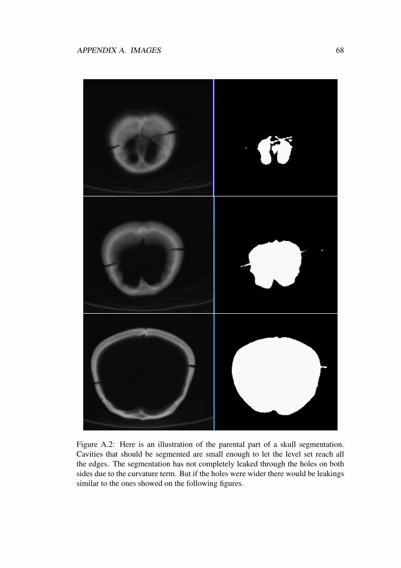
Curvature forces the resulting level set model to have less surface area and thusprotect negative effects like leaking into unwanted places shown in the figure 4.5.Note: if α = β = 0, the result is the same as flood-fill method result because there isonly the speed term taking place in the calculations.


ModelContracts

ModelExpands

T TTlow himid

pixel values

function valuesFigure 4.4: Gray rectangle encloses interval where the speed function is positive,i.e. the model expands. The fastest expansion is in the Tmid point

Figure 4.5: Illustration of leaking artefacts. Initial level set - circle (left). Withoutcurvature forces, segmentation leaks into unwanted places (center). Segmentationwith curvature forces (right).


We omitted the edge term so there are only two parameters in our method. Tun-ing of the term weights has to be performed in order to have the best results.

4.3.5 Level set methods on streaming architectures

There were some attempts for porting level set method onto special stream device.There are some obstacles due to streaming architecture that has to be overcomed toefficiently solve the problem. Firstly the streams of data must be large, contiguousblocks in order to take advantage of streaming architecture. Thus the points indiscrete grid near the level-set surface must be packed into data blocks that canbe further processed by streaming processors. Another difficulty is that the levelset moves with each time step, and thus the packed representation must be quicklyadapted.

For example Cates at al. [11] or Lefohn at al. [13] ported level set segmentationmethod to GPU. GPU is a streaming architecture with many, nowadays hundreds,of streaming cores. They run short programs called shaders. In porting to GPU ar-chitecture a texture memory is used to store input data in a large continuous block.Actual computation is then managed by vertices that flow into the shader and playa role of pointers to the texture memory. This is some kind of trick because the tex-ture memory is not addressed directly by address number like in single dimensioncontinuous address space in common processors but instead by a 2D coordinatevector. Because vertices comes as 3D points, virtual memory system that map 3Dvertices to 2D texture coordinates has to be created. Such system proposed Lefonhat al. [13]. See the figure 4.6.

Another workaround has to be performed when computed data is transferredback to the CPU. This direction is much slower than the CPU to GPU directionand thus the results has to be somehow packed. Lefonh at al. [13] describes thispackaging as well. There are although some advantages. One is the high count ofthe processors and extreme fast dedicated memory so the results can be impressive.Another is that the calculation can be directly visualized by the GPU.

Although the Cell/B.E. has some parts of the approach in common with GPU itneed not to overcome the GPU obstacles. For instance no virtual memory systemneed to be implemented because the SPE has its own flat address space by default.Also the result packing for sending back to CPU is not necessary because transmis-sion of data from and to SPE has the same speed and can be performed directly.All these Cell/B.E. processor features could result easier and more straightforwardprocess of porting of level set method. But speed of the Cell/B.E. result will notprobably exceed the GPU solution speed.


Figure 4.6: Illustration of virtual memory system (taken from [13]). 3D space levelset domain (that incoming vertices come from) is mapped via page table to 2Dtexture coordinate system.

Chapter 5

Design and implementation

This chapter will describe details of implementation and design of our test appli-cation. It will start with listing of used frameworks continuing with description ofthe process of the test application incorporation into the frameworks. After that re-sults of profiling of the application will be summarized. Followed by a new designdescription which was necessary due to unexpected profiling results. The rest ofchapter will present actual porting process with all its problems, solutions, recom-mendations and all the usable information that we discovered during the portingprocess.

5.1 Original idea of the porting process

We wanted to follow the common scenario of porting process as described in 3.5.1.In our case this means:

1. choose base implementation

2. clean it up

3. port it to PPE

4. profile it to find hotspots

5. offload hotspots to SPEs and right away to use multi-buffering technique forDMA transfers

6. optionally try some optimization steps if the results were not satisfactory

40

CHAPTER 5. DESIGN AND IMPLEMENTATION 41

5.2 Chosen algorithm and frameworks

We decided to choose sparse field algorithm of level set solving for porting toCell/B.E. It is a quite complex image processing algorithm that could test theCell/B.E. programming as a whole.

We took ITK [12] implementation of the algorithm as a base. Therefore we hadto get familiar with this huge project. It contains many algorithm implementationsas well as necessary infrastructure content such as loading and saving variety offormats. The base concept of this project is a pipeline and filters.

To get some work done a pipeline has to be build from filters. Filter is an entitythat represents an algorithm. When a pipeline is created the last filter is started.Starting event then propagates towards the beginning of the pipeline where actualcomputation starts. Output from one filter is input of the following one. Filters thuscreate a building blocks for a more complicated method.

After several first test with examples and tutorials we wrote our own testingapplication (originally with code name ’pok’). It was able load an image, run alevel set filter and save the results. Some reasonable parameter values were foundwith the pok application. It was controlled via bash scripts that is not much easynor user friendly solution. There was also no way how to visualize the results.Therefore we decided to use another framework to overcome these problems, theMedV4D project [16].

This project was originally started as a software project and is basically frame-work for creation of medical applications. Its purpose is to simplify the process ofGUI creation as well as actual computation model design. It let the programmerto focus only on actual problem solution. Filter is the basic building block as wellin this framework. Filters can be composed into pipeline just like in ITK. But theMedV4D filters are more low-level and thus faster than ITK ones. The pipeline thenoffer some implicit locking of data set parts to allow parallel computation.

5.3 Incorporation into MedV4D framework

The most convenient way how to use an ITK pipeline that can be run on theCell/B.E. seemed the client/server architecture. The part of the application thatis to be run on the Cell/B.E. is a server. While client part loads initial data or savesthe results, visualize the results and act as GUI with controls for parameter setting.

Whole process can be described as following: a client loads the input data sendsthem to a server and waits for results. As soon as the results are read back they arevisualized. Then the result can be saved or sent to the server again for computation


Load data tune params

send to server

Server computation

Save data visualize resultsresult ok result bad

Figure 5.1: Client acts like a GUI for the server side that performs actual computa-tion

with another parameters. See the figure 5.1 showing how the application with codename ’LevelSetClient’ works.

There were two main goals which were necessary for incorporation pok appli-cation into MedV4D framework:

1. Remote computing infrastructure

Infrastructure for sending commands to server along with data or parametervalues as well receiving response messages along with resulting data had tobe implemented into the MedV4D. It lead into designing whole new libraryof the MedV4D called remote computing (RC). On the client side there is aremote filter that encapsulates the whole infrastructure necessary for sendingof a pipeline to the server as well as the result handling. The server side hadto be designed completely as a whole.

2. ITK integration

This is performed by a wrapper MedV4D filter that is connected into theMedV4D pipeline. Within this filter there are two ITK images that serves asinput and output for inner ITK pipeline. Actual data of this ITK images pointto data of the wrapping MedV4D filter (see figure 5.2 for details).


INPUTdata

OUTPUTdata

INPUTMedv4Dimage

OUTPUTMedv4Dimage

ITK pipeline

ITK wrapping Medv4D filte

INPUTITK

image

OUTPUTITK

image

Figure 5.2: Basic elements are the two ITK images whose data are actuallyMedV4D images’ data

5.3.1 Client part

As mentioned above the base element of client RC part is a remote filter. It imple-ments actual command sending and result receiving functionality. It is derived froma pipeline MedV4D filter so it can be added into a pipeline and thus represent a partof the pipeline that run on a remote server. Listing of commands that the remotefilter issue to the server follows:

1. CREATE

This command is a create request. It identify the type of the filter that theremote filter represents and that should be instantiated on the server side.Server parses the command message and instantiate appropriate filter alongwith the whole pipeline (remote pipeline).

2. DATASET

Tells the server to read actual data set that the computation will be performedon. The data set is parameter of the command.

3. EXEC

This command requests actual execution of the remote pipeline. But filter pa-rameter values should be parsed before the actual execution. These values arewithin the only parameter of this command. After the parsing and associationof the filter parameters with the actual filter the remote pipeline is executed.

Purpose of the commands is to divide actual execution into stages and thus todefine a state of remote execution. This is because it would be worthless to sendactual data set to server again when user wants to execute the remote pipeline againwith the same data set but only with different parameters. Commands allow this


PrepareOutputDataset

CREATE command

ProcessImage

DATASET command

EXEC command

IN data chaged

parameter tunning & pipeline execution

server

server response processing

exit

data

filter propertie

Figure 5.3: Shows three basic states of a remote filter and when particular com-mands are sent to a server.

because remote pipeline has a state telling ’data already received, now waiting forEXEC command as many times as wanted without no more input data transmis-sion’.

The MedV4D pipeline filter defines also some stages that the behaviour of re-mote filter benefits. One of them is a method that is called only when input datachanges (PrepareOutputDataset). This is perfect place to send DATASET com-mand to server. Because this is called only on input data change thus DATASETcommand will be issued on input data change as well. CREATE command has to besent before the DATASET command to build the remote pipeline before data set istransmitted. CREATE command is sent with DATASET command because remotepipeline has to be recreated every time a new dataset arrives.

The EXEC command is sent within a function that is called when the pipelineis executed making actual computation started (ProcessImage). Whole cycle showsthe figure 5.3.

Server’s response can be either OK or FAILED. In case of OK resulting data setis received in contrast to FAILED case when no data set is expected.


accept

deserialize ident. & build pipeline

run pipeline

accepted

deser. DS prop. & connect to pipe.client

send results to client

CREATE

DATASET

EXEC

wait for DATASET command

wait for EXEC command

discard pipe & reset

on exception

client disconnected

on exception

client disconnected

Figure 5.4: Illustration of server state diagram. The states correspond to the com-mands that are accepted by the server.

5.3.2 Server part

Server part is counter part of the client one so the design reflects this. Goal of serveris to sit and wait for an incoming connection. One connection means one session ofcomputation. Currently only one session at a time is held. In context of a sessioncommand from the connected client are parsed and appropriate actions performed(see figure 5.4).

Like in every client/server application some kind of stubs are needed. In ourapplication serialization and de-serialization methods are the stubs. Goal of themethods is to ensure that the data that the client sends will be received in exactlysame order and data types.


Good example is the CREATE request. In this request identifier of remote filteris sent along with filter class template parameters identifiers. In case of mismatchof that identifiers completely different class would be instantiated on the server sideHierarchy of virtual methods of data set classes defines interface for such stubs.Interface of remote filter properties class hierarchy does the same for the remotefilter.

Another issue is endianess. Endianess identifier is sent along every command.On the other side is made decision if byte swapping should be performed. Thisallows to perform byte swapping only when it is really necessary.

Currently only one remote filter is implemented - the level set segmenta-tion. But other filters can be easily added by appending one switch branch inremoteFilterFactory.cpp source. The level set segmentation filter is implementedas a successor of ITK filter that contains appropriate ITK pipeline. This pipeline isthe most interesting part related to this work so the further content will decribe it.

5.4 Level set segmentation pipeline

This pipeline contains three ITK filters.

1. fast marching filter

Is responsible for initial level set computation. Parameters of this filter arepoint ~x in data set and distance d. Output is data set of distances from a ballshaped object with centre in the ~x with radius d. This data set is the initiallevel set front.

2. level set segmentation filter

Performs actual level set segmentation method. Parameters of this filter arethreshold interval, maximal count of algorithm iterations, curvature and speedscaling (explained above).

3. binary thresholding filter

Purpose of this filter is extract resulting object. It is thresholding that selectpixels with values less that zero that corresponds to inner part of the resultinglevel set.

The fast marching and binary thresholding filter have not been changed andare used as is part of the ITK framework. The only filter that has been changedwas the level set segmentation (LS) filter. This filter performs the sparse field levelset solving algorithm we have chosen to port to Cell/B.E.. This algorithm useslinked lists to represent the sparse field layers. The actual algorithm, as described


higher (4.3.3), is implemented in several classes. These classes form an original LShierarchy (OLSH).

5.5 Pre-porting steps

Due to the mapping of the algorithm to Cell/B.E. and due to poor lucidity and highuniversality of the ITK code radical changes were necessary. We decided to rebuildappropriate part of the OLSH responsible for the sparse field level set computation.Our own LS image segmentation filter should be the result of that changes.

There are actually two class hierarchies in the OLSH. One represents the filterthat performs level set algorithm, the filter hierarchy. And the other computes theFDE using the upwind scheme [15], the finite difference function hierarchy.

At the top of the function hierarchy there is FiniteDifferenceFunction that com-putes the upwind scheme with assistance of virtual methods that are implementedin successors. Successors are:

1. LevelSetFunction

It provides curvature term computation methods.

2. SegmentationLevelSetFunction

It manages speed image computation infrastructure.

3. ThresholdSegmentationLevelSetFunction

It computes actual speed image.

The base of the filter hierarchy is FiniteDifferenceImageFilter. It computes themain loop of level set calculation (see step 1 in 4.3.3). Virtual methods of its suc-cessors are used to implement the appropriate sub steps.

The first successor is the SparseFieldLevelSetImageFilter provid-ing implementation of algorithm’s Step 1a through the update cal-culation function. Other steps are performed by the apply up-date function. Next successors SegmentationLevelSetImageFilter andThresholdSegmentationLevelSetImageFilter only manage difference functionin appropriate manner. The ThresholdSegmentationLevelSetImageFilter calculatesspeed function as described in 4.7. The function is computed at the beginning forthe whole data set into pre-allocated image. This image is another notable amountof memory that cannot be accepted for our purpose (see paragraph B.4).


Figure 5.5: Illustrates the original ITK FiniteDifferenceFunction hierarchy and theFiniteDifferenceImageFilter hierarchy and their relationship

Our approach calculates the speed function every time it is needed without anypre-calculations. This approach could be possibly better for the Cell/B.E. streamingnature.

We have simplified these two hierarchies. One reason of the simplification wasthe removal of the pre-calculated image. The other one was code clean-up andrefactorization. Result of these changes is our own filter (ThreshSegLevelSetFilter,OOF). It omits all unnecessary part of the OLSH and uses reasonable parts of theoriginal ITK level set segmentation filter (see the figure 5.6). It is also ready to beported for the Cell/B.E.

In the function hierarchy only the base class that the resultingThresholdLevelSetFunc class is derived has left. This new class does thesame job as original LS function hierarchy and omitts the pre-allocation of thespeed image. The computation of particular up-wind scheme terms was separatedinto standalone classes for more code readability and modularity.

The filter hierarchy was shortened and begins already inSparseFieldLevelSetImageFilter. All its successors in the original hierarchywas omitted since they did anything reasonable for our purpose. Some functionimplementation from the SparseFieldLevelSetImageFilter was borrowed into thenew OOF to be ported for the Cell/B.E.


Figure 5.6: Show result of original LS hierarchy rebuilding. Some unnecessaryparts was omitted to clean-up the code and to change behaviour towards a streamingarchitecture as well as the term computation was separated into supporting classesfor modularity

Profiling resultsfunction name subroutine time spend percent

in calculations %(in seconds)

ApplyUpdate() 20.15 75.21PropagateAllLayerValues() 16.64 62.11UpdateActiveLayerValues() 2.27 8.47

CalculateChange() 6.11 22.8ComputeUpdate() 3.97 14.82

TOTAL 26.79 100

Table 5.1: Results of profiling showed that ComputeUpdate step that was originallythought to be hotspot takes only 14.82% of computation time.

5.6 Profiling

As the first step of the porting process the server application with the OOF withinwas build and profiled with following results:

The profiling results (see Table 5.1) show that the most time consuming part ofthe program is not the difference solving in update calculation step but the updateapplication step. The original idea was to offload only the difference solving withinthe update calculation step which is performed on 33 voxel matrix and calculatedindependently of the others which makes this job perfectly suited for offloading tothe SPE. But the time necessary for computation of this part is only the fragment ofthe whole. This is the reason for another changes to the OOF.


MySegmtLevelSetFilter

Initial level set comp.

Intial layers comp.

SPE program manager

SPE program

UpdateCalculator

ApplyUpdateCalculator

Figure 5.7: Diagram of new design components. Calculation of only the initialstates is performed by the PPE. The rest is moved to the SPEs through the SPEM-anager that perform all necessary steps to run the SPEs.

5.7 New design

Actually the whole OOF had to be rebuild and from original ITK class hierarchylast nothing. Everything replaced by the OOF and our own version of originalFinititeDifferenceImageFilter (FDIF) where the main loop of the algorithm as wellas stopping conditions resides. The reason of replacing even the FDIF is that itsuppose usage of a difference function and its virtual methods. But in the newdesign the difference function is offloaded to the SPE so it was taken out completelythrough the FDIF.

In the figure 5.7 can be noticed that almost whole original ITK pipeline is of-floaded to SPE. Only initialization routines are left to the PPE. This lead to createthe SPE program manager that will manage computations on SPEs. It is responsiblefor SPE thread initialization and run, and SPEs synchronization.

SPE part consists of two main parts. The UpdateCalculator, performing updatecalculation and the ApplyUpdateCalculator, performing update application. TheUpdateCalculator traverse over layer0 and computes update values for its points. Itperforms STEP 1 of sparse fields algorithm 4.3.3. The computed values are storedin a update buffer.

Then is the ApplyUpdateCalculator’s turn that performs the rest of that algo-rithm on the calculated update values within the update buffer. In context of ourimplementation the particular steps mean:

• STEP 2

For every layer0 compute new level set value and perform the test if it staysin the interval [-1

2 ,12 ]. If not, move the point into appropriate status list. This

is performed by the UpdateActiveLayerValues method.


• STEP 3

Is performed by sub-component of the ApplyUpdateCalculator, theLayerValuesPropagator. This traverses over all layers, process their valuesand remove nodes if they are no longer in a layer. Step processed by thePropagateAllLayerValues.

• STEP 4

Traverse over status lists in innermost to outermost order and process theirnodes. A node is moved to inward (outward) status list and simultaneouslyappropriate layer if needed. This is performed by the ProcessStatusListsmethod.

5.7.1 Data flow

In porting process is necessary to know the data flow i.e. find out what data are sentand where. What data are there produced and especially the size of all the data.This is because of decision where they will be stored. Whether in the SPE localstore or in the central memory. For the first case their size has to be limited becauseof limitation of the local store. For the second case a communication via DMA willbe necessary but the data size is not limited.

There are both cases in our application. The ProcessStatusLists method can beperformed completely within the SPE without loading any data from the centralmemory. But the rest of processed data is too big and can not reside within the SPE.It has to be DMAed in chunks from the central memory. The big data are statuses,actual level set values and features that are stored within status, output and featureimages. So it is necessary to load and store parts of that images. Computation isperformed on small neighbourhood of voxels 3x3x3 (neighbourhood). So 27 voxels(resp. statuses) has to be transferred for one node processing. Another big data arenodes within actual layers which are linked list chains of nodes. Traversal overthe chains is performed sequential by loading one node after another. For eachloaded node one or more neighbourhoods shall be loaded. The computation is thenperformed on those neighbourhoods.

There are other data that have to be stored within central memory and that con-tribute to the data flow as well. Next list describe what data are processed in mostimportant methods resp. steps within our application:

• UpdateCalculator

It needs an array which is as long as the layer0. The size of the layer can bevery big so it is impossible to store it within SPE local store. Therefore thearray has to reside in central memory and its content has to be load into SPElocal store buffer while the list traversal.


• UpdateActiveLayerValues

It process the array from UpdateCalculator so it has to load it from the centralmemory. It operates on layer0. Some nodes are moved into status list andsimultaneously UNLINKed from layer0 list. Layer resides in central memoryso beside the loading nodes for traversing, some special operation has to bedefined on the layers which perform the UNLINK action.

Status lists are temporary objects. They live only during oneApplyUpdateCalculator turn. So they can reside within SPE’s local store.Therefore no special operation communicating with the central memory hasto be defined. But processing of the list0 has to be changed. In original ITKcode the UpdateActiveLayerValues operates on the whole layer0. One call tothis method can produce too long status list that would not fit into the localstore. So iteration over layer0 has to be limited to produce limited lengthstatus lists. We have defined the limit with constant MAX TURN LENGHTand call processing the limited segment of the layer0 a ’turn’.

• ProcessStatusLists

It works on the limited length status lists. During the lists processing somenodes are moved from one to another layer which means they have to be un-linked from one and linked into another. Linking into another layer definesanother layer operation, PUSH. One status list is processed untill it is emptytherefore all status lists remain empty and thus ready for the next UpdateAc-tiveLayerValues turn after the ProcessStatusLists method finishes.

• PropagateAllLayerValues

This method traverse over all the layers and performs moving nodes amongthe layers. This means operations PUSH and UNLINK as well as layer traver-sal and appropriate neighbourhoods loading.

There are some actions and operations defined above that need communicationwith the central memory. These are parts of the program where PPE - SPE commu-nication features of the Cell/B.E. take place. Other SPE code need not to know ifit is run on the SPE or the PPE. Therefore set of tools that performs the PPE - SPEcommunication was developed.

5.7.2 Tools

Tools are parts of the program that perform data transfer between the PPE and theSPE. All these tools perform multi-buffering to avoid waiting for data.


1. NeighbourhoodCell

Represent the part of an image (33 voxel matrix) needed for one node com-putation. It uses DMA transfer list that allow data handling in scatter-gathermanner. Neighbourhoods are grouped within PreloadedNeigborhoods con-tainer that manages which neighbourhood is being loaded, used in computa-tion or saved i.e. actually performs multi-buffering.

2. RemoteArrayCell

Represents an array stored in the main memory. This tool is usedfor the UpdateCalculator to save computed update values and in theApplyUpdateCalculator to retrieve the values which the UpdateCalculatorhas stored. Its role is to perform DMA transfers not for every single valuesave but on a buffer of that values.

3. LinkedChainIteratorCell

It traverse over a layer which is linked list data structure. As soon as one itemis retrieved, transfer of the next one is immediately started before the retrieveditem is processed letting the started transfer complete before the loaded itemprocessing finishes.

PUSH and UNLINK operations are related to linked chains of nodes, the layers.We decided to implement them using mailboxes. Mailbox is another SPE to PPEcommunication channel which is able to transfer 32bit integers synchronously.

Because of the 32bit integers transfer limitation actual PUSH and UNLINK pa-rameters have to be decoded and encoded.

1. PUSH

Has to push a node into specified layer. Node coordinates and number oflayer is encoded and sent over mailbox to the PPE. On the other side the PPEcreates a new node appropriately according decoded coordinates and puts itinto specified layer.

2. UNLINK

Operation has to unlink a node from a specified list. Address of the node andthe layer number are the parameters. Address is transferred in 32 bit chunks(because mailbox has 32 bit size) which are decoded on the PPE side to actualnode address that is then unlinked from specified layer.

Another support tool that is worth mentioning is ObjectStore which is simplememory allocator templated with class of item it provides and size of an array thatthe items are taken from. Provides two main methods, Borrow and Return. It is


used for allocation of status layer nodes. They reside in the local store and thusshould be allocated on the stack.

Great advantage of the tools is also that the whole code uses only the tools forthe central memory communication. Therefore debugging transfer issues meansdebugging the tools.

5.7.3 Work balancing

The sparse field layers are the central part that defines the amount of work to beperformed. So it is necessary to balance their length among the SPEs that processthem. This work is left to Work manager. Its goal is to ensure that all the layers aredivided among SPEs uniformly.

For this purpose the UNLINK and PUSH operations implemented using mail-boxes fits well. The idea behind is that actual operation on the linked list is dele-gated to the Work manager. It decides which SPE layer segment should be the nodeappended into.

The whole process can be compared with a company department where areseveral workers doing actual work and where is one manager who distributes thework among the workers.

5.8 Actual porting process

Here we will describe our experience with actual porting procedure, problems thatthe procedure has brought and our solutions of those problems.

5.8.1 PC as Cell/B.E. simulator

Because remote debugging program running on PS3 is quite time consuming i.e.seconds for step into command and the like and because of small amount of mem-ory (see paragraph B.4) we decided to left actual porting to the very end of theprocess. Features that are needed for running on the SPE were gradually added intothe original code. Some parts were rewritten e.g. the UpdateActiveLayerValuesturn to allow some data to live in the SPE’s local store. All the changes have notchanged the programs’ output, so one can say that the all the programs in everystep were equivalent. All the debugging was performed on PC platform locally andthus quickly. The Cell/B.E. special features like DMA transfer was simulated bythe memcpy function or the mailbox issues trough a simple queue.


5.8.2 Moving to PPE

It seems that moving the code to PPE is easy and there could be no problem. But wefaced a problem that is worth to mention. Because our code uses a lot of third partylibraries there are quite much paths to include folders. It is necessary to managethem well and not to mix architecture dependent ones.

We have mixed up include files of the boost library when cross-compiling andexperienced a totally strange behaviour. We thought that we can use boost libraryincludes that come from repository for i686 architecture. The code crashed on boostcode that should be debugged and stable. For instance opening a file has crashedfor an unknown reason. When program was compiled with includes from ppc(64)repository all the problems have disappeared.

5.8.3 Tools porting

Next step was to port the tools for SPE. In fact is to rewrite usage of memcpy thatsimulate the DMA transfer to use real DMA transfer.

Data that are transferred through DMA (DMAed) within the Cell/B.E. shouldmeet size and align conditions (see [5], Chapter 4). Data that does not meet thiscondition will generate a BUS error. This condition force that all data that are beingDMAed should be allocated to aligned addresses (see objectStore.h or updateVal-sAllocator.h).

Debugging within this step have been performed already on a Cell/B.E. ma-chine. We used both PS3 and systemsim. Systemsim can detect which DMAtransfer brakes align rules and thus cause the BUS error but it is really slow. In-stead using systemsim we have implemented a DMAGate (see DMAGate.h) that allDMA transfer go through and where are all the conditions checked. Such centralpoint for all DMA transfer is really important part of Cell/B.E. program because itgathers all DMA stuff into one place making debugging much more easier.

5.8.4 Memory checking tools

Gradual code porting for SPE was really time consuming due to fact that toolsoperates with a stack memory. Debugging such parts needs extra care for whatis where rewritten. Since a stack memory is used some part of call stack wouldbecome corrupted and the program becomes undefined. The worst thing is thatit can continue without crash or to crash on totally different place. Errors of thistype are always hard to track. There is need of usage of some memory checking


tools. For us memcheck tool, part of Valgrind, proved to be useful to detect stackcorruptions.

Usage of DMA transfers (or memcpy) is also dangerous. It rewrites destinationmemory without checking what is within that memory. Then many errors causingsegmentation faults arise.

We have spent lots of time debugging plenty of such errors. Even in resultingapplication can occur some errors of this kind. Debugging every single this kinderror is a never ending story. So we recommend either to develop additional toolsthat will check such errors or to use memory checking software such as Valgrind [8].We used the Valgrind but not from the beginning. So when we check the programthere was too much warnings of the same kind. Solving them was impossible inthat time.

Checking the program with memory checking tools is necessary already fromthe very beginning of the development and quite often. It is advisable not to makehuge code changes not only due to memory checking but due to actual processas such. It is better to develop gradually in a small steps. One can then find anerror more simply. This is universal rule for programming but we believe it is validspecially for the Cell/B.E. porting process.

Chapter 6

Results

In this chapter speed measurements of our application will be presented as wellas a few pictures of the results. Because we have not accelerated the computationover traditional processors a discussion of the reasons will follow. We will mentionpossible changes in design to speed up the execution. Then some considerationhow shall the algorithm that is well suited for the Cell/B.E. look like. Chapter willbe finished with comparison of complexity of programming for the Cell/B.E. andconventional processors.

6.1 Speed measurements

Actual speed measurement is performed within GenerateData method of theFiniteDifferenceFilter. Counter is started right after initialization phase i.e. be-fore main algorithm loop and stopped right after the loop. The program memoryusage was tuned to use only really necessary amount of memory within the mea-sured interval. Valgrind’s massive tool was used for the memory usage tuning. Thiswas necessary because of the PS3 limited memory, see paragraph B.4

Beside the server memory usage tuning other changes was made also within theclient part. There has been a special filter developed. The filter shrinks a data setto a given size and cast its voxels to float. The shrinking is performed by a linearinterpolator. The purpose of the float casting is avoidance of allocation of additionalmemory on the server side that would be necessary for float data set.

It is strange that the command top shows far bigger memory usage than theValgrind’s massif. We have not cared much about it but the idea is that the topshows all memory requested from the system while the massif shows exact memoryused by the process.

57

CHAPTER 6. RESULTS 58

Measurement resultsdata set size seed init. max. arch. time

dist- itera- spendance tions (sec)

3slices 512x512x3 [256,256,1] 40 800 Cell/B.E. 16.48(skull 1) i686 . 1.89skull 1 256x256x80 [128,110,20] 20 500 Cell/B.E. 471.89

i686 95.23skull 1 256x256x80 [128,110,20] 4 500 Cell/B.E. 325.93

i686 61.74skull 2 256x256x80 [128,110,20] 4 500 Cell/B.E. 319.47

i686 55.88skull 2 256x256x80 [128,128,40] 4 500 Cell/B.E. 366.63

i686 76.9

Table 6.1: Results of speed measurement. The first difference is a bit big probablybecause of the small data set and insufficient time to take advantage of parallelismof six SPE. The second measurement shows that the PC implementation is aboutfive times faster. The rest of measurements, performed on different data set andparameter configurations prove the coefficient five.

Results of the speed measurement is summarized in the table 6.1. Every mea-surement was run with the same curvature and speed-scaling factors. But with dif-ferent initial distance, maximum iterations and seed parameters. These parameterswere set according to data set size.

Three different data sets were measured. All of them was CT images of a skullthat were scanned for anthropological purposes. Measurement of some volumet-ric parameters of such images is a valuable source of data for the anthropologist.Method implemented in our application could be used in the praxis for such pur-poses if the application is quick enough. Therefore speed-up of the current methodsis necessary.

6.2 Reasons of slowdown and possible improvements

Porting the code to run on SPEs and distribution of the calculations among theavailable SPEs is not sufficient to get more speed from the Cell/B.E. over traditionalprocessors. The optional speed-up porting phases are necessary to be performed.But our program has another speed pitfalls.

The biggest problem is the CellNeighbourhood that represent a small part of animage (the 33 voxel matrix). It is transferred for every layer item. In some parts


1 2 3 4 ...

1 2 3 4

quadword

...

central memory array

LS array

word (32 bits)

Figure 6.1: Illustration of transfer of data that are smaller than quad-word. Hard-ware automatically increases address within the local store buffer in such way thatevery transferred item is quad-word aligned.

1 2 3 4 ...

1 2 3 4

quadword

...

central memory array

LS array

word (32 bits)

list 1 (1st word within quadword)

list 2 (2nd word within quadword)

list 3 (3rd word within quadword)

list 4 (4th word within quadword)

...

Figure 6.2: Workaround for transfer for smaller than quad-word chunks. It usesmore than one DMA list. One per quad-word align e.g. for chars 16 DMA lists areneeded.

the both output and status image neighbourhoods are transferred. We wanted toperform the transfer in scatter-gather manner through DMA lists but we have facedsome problems. The DMA transfers and specially using DMA lists are designed forbig amount of aligned data. When they are used for small amounts (smaller than16bytes per list item) performance goes down because of unaligned data transfer.When smaller than 16 bytes (quad-word) data are being transferred every singleitem is automatically aligned to quad-word address within the local store buffer(see figure 6.1).

This increase required size of a buffer that is needed for the transfer. This canbe partially solved by usage of multiple DMA lists (one for each quadword align).This is illustrated in the figure 6.2. For details see [10].

We have adopted this workaround and used it within the neighbourhood transfer.Because of the automatic local store quadword address aligning we had to use atranslation table. This table maps position of actual neighbourhood members into


Figure 6.3: Comparison of one slice segmentation on different architectures. Theleft was computed on PC (i686), the right on Cell/B.E. Although the segmentationwas run with the same parameters there is small difference between those two im-ages. The Cell/B.E. level set has not reached as far as the PC one. It is because ofduplicate nodes within layers.

position within the local store buffer. This is working solution but overhead isincredible and thus the solution is useless (see cellNeigbourhood.tcc for details).

Another problem is order of layer nodes resp. neighbourhoods processing.When there are two nodes within one layer that are next to each other processedsubsequently changes made to the first processed neighbourhood would not appearto already preloaded next one. Therefore another merging was necessary to beperformed. This coerced another changes to neighbourhood transfer and made theactual transfer unbearably expensive operation.

Another pitfall is the situation when sibling nodes are processed by two differ-ent SPEs. Adding nodes to layers is based on information from neighbours of thecurrently processed node. So it is possible that two different SPE inserts the samenodes subsequently into one layer because they process sibling nodes i.e. overlap-ping neighbourhoods. This makes no changes to output but means additional over-head due to processing multiplied nodes. Solution to this problem would requiresynchronization among the SPEs.

Additional improvements of neighbourhood transfers should be done to speedup the execution. This corresponds to data transfer optimization step of portingprocess (see paragraph 3.5). In our case this would mean radical simplificationof neighbourhood transfer. This transfer should take only a few instructions to beeffective. In the SDK examples transfers are performed by simple macros whichis probably the most effective way. In our case simplification if the neighbourhoodtransfer would mean utilization of bigger image part transport within a single DMAtransfer to avoid automatic local store alignment. This would mean a bigger local


store array to store the image part. But processing of nodes that are associatedwith the part would be somehow gathered and thus the count of transfers wouldbe lower. Processing of nodes should take into account their spatial informationwhen inserted into a layer and thus to gather the node processing on the biggerneighbourhood. But such computation scheme would coerce complete redesign ofthe application and begining from scratch.

6.3 Code and design complexity

The Cell/B.E. programming means mainly programming for the SPEs because oftheir performance and count. Because of indirect memory access and need of usageof some multi-buffering memory transfer scheme the design is quite more complexover common processor. With another limitation which is the local store size isdesign of a Cell/B.E. application a challenge.

The Cell/B.E. is designed for intensive computation applications. For a pro-grammer this means utilization of all SPEs and all their features at the maximumlevel. It is only possible for certain class of algorithms. Let’s call them streamingparallel algorithm. But what is it? What is the definition? Work on our applicationhas showed us what the streaming parallel algorithm is not. Therefore by nega-tion of the features that slow down our program we could get a definition of thestreaming parallel algorithm. It would look like the following:

1. Streaming nature

Data of that program are uniform and can be processed in a small pieces(chunks) which are mutually independent and which can fit in the local storememory. This means that for a chunk processing only this chunk is necessaryand not any part of the other chunks. When this chunk is once processed it isstored and is never retrieved for processing again.

For our application this is not true. At least not for all the input data. Process-ing of a sparse field layer meets the streaming nature. But processing of partsof underlying images (neighbourhoods) associated with these nodes does not.The neighbourhoods are mutually dependent see 6.2.

2. Paralel nature

Input data can be divided into parts which are again mutually independentand which can be sent to particular cores for processing. This avoids anymutual synchronizations among the SPEs.

For our application is again not true. Work that is divided among the coresis not independent because of dependency of particular neighbourhoods. See6.2 what causes problems.


When algorithm does not meet the streaming parallel definition then it shouldnot be implemented or it must be changed. This means e.g. to use different datastructures or to change the way the current data structures are used. In our case,change of the data structure to somehow gather node processing to specific imagepart would mean change of the algorithm we implemented. But then it would notbe the original algorithm any more.

In contrast there are algorithms that fits the streaming parallel algorithm defini-tion. The examples in the SDK that meet the definition. Except them e.g. thresh-olding meets the definition as well. It operates on an image that has uniform data- pixels. It apply simple condition on each pixel which result depends only onthe processed pixel. Processing can be divided into chunks. These three featuresmeets the streaming condition. Moreover the data can be divided into independentsets that can be processed by multiple cores (the parallel nature). Implementationof this algorithm can therefore result huge performance gain on the Cell/B.E. thanconventional processors.

Our work has showed importance of the initial consideration and the designphase. When there are more algorithms that are solving a desirable problem pro-grammer should think carefully which one will be the best for porting to theCell/B.E. First stage of the initial consideration should be a model of the applicationimplementing chosen algorithm. Consideration what kind of data are processed. Ifthey are uniform. If they are divisible into chunks. If the computing can be dividedinto independent parts i.e. what entity defines amount of work to be done. Theseare questions that lead to answer if the chosen algorithm is or is not the streamingparallel. If the answer is no, implementation of that algorithm is rather worthlessand will result such a suboptimal program as the ours.

Another thing is the code complexity. Performing the optimisation porting cyclesteps utilise all the Cell/B.E. features and thus leads to gain more performance.Usage of language intrinsics, different kind of special instruction of macros forvariety of purposes, multi-buffering, etc. increases actual code complexity whereasdecreases code readability. It is also time consuming and hard to perform.

There is still another question to be answered. Is the porting of an algorithmworth at all? Since only some special machines are equipped with the Cell/B.E.actual data have to be sent to the machine for computing and results have to be sentback. Therefore only complex algorithms where performance gain would be biggerthan the time spent in transfer of actual data set are worth to port. The algorithmwe have tried to implement is complex enough to be offloaded to compute on re-mote machine while the mentioned thresholding would not. As soon as commonmachines such as notebooks, desktops are equipped with the Cell/B.E. processoreven a class of such simple image processing algorithms that is implemented ineveryday-use software such as the thresholding or variety of masking or edge de-tections is worth to port.

Chapter 7

Conclusion

At the beginning we studied available literature to find out what is actually theCell/B.E. and what benefits it brings. What special features it has and what theyare good for. Then we have been trying to install SDK to start actual developmentprocess. During this phase we faced some obstacles such as bugs, incompatibili-ties among tools, the libraries that the tools use and even the operating system vs.SDK incompatibilities. Therefore we had to go through variety of forums and othersources to find the solutions. As a side effect we improved our Linux knowledge.Eventually we managed to install SDK and was able to start developing. Thenwe have been testing variety libraries, tools and examples to get familiar with theCell/B.E. development.

We have chosen sparse field algorithm implementing level set based segmen-tation to port to Cell/B.E. platform. This is quite complex algorithm to test theplatform’s potential. We adopted ITK implementation of that algorithm. Thereforewe had to study ITK tool kit and its internals. We have also incorporated the wholeprogram into MedV4D framework. That means we have implemented new modulesthat allow using ITK and can offload some part of processing to remote machine.

Actual porting process started with cleenup the ITK code. Then profiling ofexisting application took place finding out hot spots of the code which can be inturn offloaded to SPE to take advantage of Cell/B.E.. But profiling results wasquite unexpected so another redesign of application followed. In this new designalmost whole original ITK code was offloaded to the SPE. A big code restructuringwas necessary to allow us to perform actual computations on the SPE. We haverepeatedly debugged same kind of errors due to corruptions of stack memory causedby DMA transfers. This has proved importance of usage memory checking tools.Finally we have been able to run the whole algorithm on SPE and to measure timeneed for computations.

The result of measurement showed that simple move the computation to the

63

CHAPTER 7. CONCLUSION 64

SPEs is not sufficient because it does not utilize all the Cell/B.E. features. Wehave identified some bottlenecks of the application and discussed possible solutions.Implementation of these solutions would require whole application redesign usinganother data structure. These changes would actually mean change of the usedalgorithm.

Because of complexity of the chosen algorithm and the base implementation wespent so much time with uninterresting work and in many cases we have done theporting process in wrong way. This lead to silly mistakes and another time wastingsin debugging bugs. But on the other hand the improvization was the reason ofappearing of interresting ideas like the PC as the Cell/B.E. simulator.

Our work has proven that taking an implementaion of an algorithm and gradu-ally change it to let it run on the SPE is not a good way of proting process. Insteadit is necessary to think if the algorithm is well suited for porting. And if it is thenimplement it from scratch considering all the Cell/B.E. features utilization alreadyfrom beginning. The gradually changing the original implementation with the ideaof utilisation all the Cell/B.E. features as soon as it is able to run at least on the SPEis wrong. Then it could meand the whole application redesign like in our case.

We have also discussed differences between the programming for conventionalprocessors and Cell/B.E. As well as question of actual algorithm complexity andworthiness of porting them to Cell/B.E.

The Cell/B.E. platform is very interesting for its variations of use scenarios andability of program tuning and customization. We think the pallet of tools and fea-tures of the Cell/B.E. can make it interesting alternative to conventional processorswhose lifetime is getting shorter due to limitations in manufacturing process. TheCell/B.E.’s great potential has already been proven but it is still waiting for widerspectrum of programmers.

If the process of the Cell/B.E. development starting became simpler we believemuch more new programmers would start using and programming it. Nowadaysthere are plenty of information about the Cell/B.E. but they are somehow unsortedor out of date. The best information source are documents shipped along with theSDK. But they are targeted to contain all the information regardless the level ofexperience of the reader. That means when a programmer wants to start developingapplications on the Cell/B.E. he/she would go trough a plenty of that informationbefore he/she can start actual work. It is a pity there is total lack of informationfor PS3 users within SDK documentation. This is quite problem when a majorpart of beginners has a PS3 available. There is simply lack of some ’cookbookfor beginners’ with practical information and some howtos. We believe this workcould be such a cookbook with such practical information that potentially may helpto some other programmers who would like to start developing for the Cell/B.E.

Bibliography

[1] Mike Acton. Cell performance website. www.cellperformance.com, 2009.[Online; accessed 15-May-2009].

[2] Mike Acton. Understanding strict aliasing article. http://www.

cellperformance.com/mike_acton/2006/06/understanding_strict_

aliasing.html, 2009. [Online; accessed 22-May-2009].

[3] David Adalsteinsson and James A. Sethian. A fast level set method for prop-agating interfaces. J. Comput. Phys., 118(2):269–277, 1995.

[4] Jonathan Bartlett. Programming high-performance applications on thecell be processor series. http://www.ibm.com/developerworks/views/

power/libraryview.jsp?search_by=Programming+high-performance+

applications&Submit.x=47&Submit.y=17&url=%2Fdeveloperworks%

2Fviews%2Fpower%2Flibrary.jsp, 2009. [Online; accessed 22-April-2009].

[5] IBM corp. Programmer’s guide. /opt/cell/sdk/docs/index.html.

[6] IBM corp. Cell Broadband Engine resource center website. www.ibm.com/

developerworks/power/cell, 2008. [Online; accessed 12-December-2008].

[7] IBM corp. SDK documentation. www.ibm.com/developerworks/power, 2009.[Online; accessed 14-February-2009].

[8] Valgrind developer team. Valgrind memory check tools documentation.valgrind.org, 2009. [Online; accessed 20-March-2009].

[9] Marc Droske, Bernhard Meyer, Martin Rumpf, and Carlo Schaller. An adap-tive level set method for medical image segmentation. In IPMI ’01: Pro-ceedings of the 17th International Conference on Information Processing inMedical Imaging, pages 416–422, London, UK, 2001. Springer-Verlag.

[10] Cell/B.E. forum. DMA list issues thread. http://www.ibm.com/

developerworks/forums/thread.jspa?threadID=143212, 2009. [Online; ac-cessed 24-April-2009].

65

BIBLIOGRAPHY 66

[11] Ross T. Whitaker Joshua E. Cates, Aaron E. Lefohn. Gist: An interactive,GPU-Based level set segmentation tool for 3D medical images. School ofComputing University of Utah Salt Lake City, UT 84112 USA, 2004.

[12] Kitware. ITK website. www.itk.org, 2009. [Online; accessed 4-January-2009].

[13] Aaron E. Lefohn, Joe M. Kniss, Charles D. Hansen, and Ross T. Whitaker. Astreaming narrow-band algorithm: interactive computation and visualizationof level sets. In SIGGRAPH ’05: ACM SIGGRAPH 2005 Courses, page 243,New York, NY, USA, 2005. ACM.

[14] Fedora maintainer team. Fedora project site. http://fedoraproject.org/,2008. [Online; accessed 22-December-2008].

[15] Stanley Osher and James A. Sethian. Fronts propagating with curvature-dependent speed: algorithms based on hamilton-jacobi formulations. J. Com-put. Phys., 79(1):12–49, 1988.

[16] CGG team. project MedV4D. http://cgg.mff.cuni.cz/trac/medv4d, 2009.[Online; accessed 15-January-2009].

[17] OpenCV team. Optimization strategy article. http://cell.fixstars.com/

opencv/index.php/Optimization_Strategy, 2009. [Online; accessed 21-May-2009].

[18] Ross T. Whitaker. A level-set approach to 3D reconstruction from range data.Int. J. Comput. Vision, 29(3):203–231, 1998.

[19] Wikipedia. Segmentation (image processing) — Wikipedia, the free encyclo-pedia. http://en.wikipedia.org/wiki/Segmentation_(image_processing),2009. [Online; accessed 22-April-2009].

[20] Terry S. Yoo. Insight into Images: Principles and Practice for Segmentation,Registration, and Image Analysis. AK Peters Ltd, 2004.

Appendix A

Images

Figure A.1: 3D View of the segmented data set. VTK viewer used to visualize thedata set. On the left part there is the parietal part of the skull. This part is quite wellsegmented as illustrate the figure A.2 The segmentation of the front skull part (onthe right side) is poor due to leaking through the eye sockets (see the figure A.4).

67

APPENDIX A. IMAGES 68

Figure A.2: Here is an illustration of the parental part of a skull segmentation.Cavities that should be segmented are small enough to let the level set reach allthe edges. The segmentation has not completely leaked through the holes on bothsides due to the curvature term. But if the holes were wider there would be leakingssimilar to the ones showed on the following figures.


Figure A.3: This image set shows middle slices of the skull data set segmentation.Some edges are reached by the level set (on the right side of the skull mostly) whilesome are not. This is caused by insufficient count of algorithm iterations (500) orimproper initial level set placement. It proves that result is highly initial parameterssetting sensitive.


Figure A.4: These three images illustrate the leaking of level set through throathole, cavities near nose and eye sockets.


Figure A.5: This slice is really poorly segmented due the leaking of the level setthrough the previous slices (see the figure A.4).

Figure A.6: The original skull data set was blended (the red background) with theresult of segmentation (the bluegreen overlay).

Appendix B

Tools setup

This part is a cookbook how to install all the necessary content to be able to begindevelopment for the Cell/B.E. It also covers some bugs fixing as well as useful hintshow to use the partial SDK content. The instruction concerning the SDK installationwas based on installation on a i686 machine. But shall be the same for the otherarchitectures since it operates on the same operating system and repository versionsof third party software.

The first step is installation of Fedora operating system. For details see fedoraofficial site [14].

B.1 SDK installation

As first you have to do is to download actual SDK. Go to http://www-128.ibm.com/

developerworks/power/cell/downloads.html?S_TACT=105AGX16&S_CMP=LP. Youshould download following files:

1. SDK 3.1 Installer cell-install-3.1.0-0.0.noarch.rpm (11MB), contains installscript and other stuff for SDK installation.

2. SDK 3.1 Developer package ISO image for Fedora 9 CellSDK-Devel-Fedora 3.1.0.0.0.iso (434MB), contains rpm packages that actual SDK iscomposed from (SDK packages)

3. SDK 3.1 Extras package ISO image for Fedora 9 CellSDK-Extras-Fedora 3.1.0.0.0.iso (34MB), contains some extra packages for Fedora

Download it wherever you want (even though in documentation is /tmp/cellsd-kiso). Lets call the folder ISODIR. First you shall stop the YUM updater daemon.

72

APPENDIX B. TOOLS SETUP 73

/etc/init.d/yum-updatesd stop

If it outputs: ”bash: /etc/init.d/yum-updatesd: No such file or directory”, you donot have any YUM updater daemon installed so you can skip this step. Now issuefollowing command to install required utilities for SDK installation

yum install rsync sed tcl wget

Now install the downloaded installation rpm.

rpm -ivh ISODIR/cell-install-3.1.0-0.0.noarch.rpm

After this step you have new stuff in /opt/cell installed. There is SDK instal-lation script (cellsdk) located as well. It is wrapper for YUM that manages the SDKpackages. Run it with parameter –help to see the usage. So next step is to run it.

/opt/cell/cellsdk --iso ISODIR -a install

Parameter –iso tells to use the downloaded ISOs and path where they can befound for mounting onto a loop-back device. Parameter -a disables agreeing li-censes. Otherwise you have to write some ’yes’ to agree. Process begins withsetting local YUM repositories pointing to the ISOs. Then all default packages areinstalled with all their dependencies. To check result of the installation issue

/opt/cell/cellsdk verify

Now we have SDK installed. Lets continue with installation of IDE. It consistsagain of packages. Now install yumex that provides graphical interface to YUM tosimplify processing packages. It let you simply check packages that you want toinstall.

yum install yumex

To install CellIDE run yumex, go to Group View→Development→Cell Devel-opment Tools. Check cellide, that is actual IDE (Eclipse with cell concerning stuff)and ibm-java2-i386-jre, that is Java Runtime Environment, JRE needed for runningof the IDE. Click ’Process Queue’. Note: you should have the ISOs mounted onto aloop-back device. Otherwise you get ’Error Downloading Packages’ after clicking’Process Queue’. Therefore you have to mount ISOs whenever you want to installpackage concerning the SDK


/opt/cell/cellsdk --iso ISODIR mount

After the installation you have two new folders. /opt/cell/ide that containsthe IDE and /opt/ibm/java2-i386-50 where the JRE resides. To run the ide youhave to specify folder where the JRE is (through -vm param).

/opt/cell/ide/eclipse/eclipse -vm /opt/ibm/java2-i386-50/jre/bin/

B.1.1 Bug fixing

If you start the IDE and it crashes with unhandled exception it is probably causedby xulrunner library. It is usually installed with Firefox3. There is followingworkaround:

1. download an older version of the xulrunner

e.g. from: http://releases.mozilla.org/pub/mozilla.org/xulrunner/

releases/1.8.1.3/contrib/linux-i686/xulrunner-1.8.1.3.en-US.

linux-i686-20080128.tar.gz

2. untar to an accessible directory

Lets call it XULDIR.

3. edit the

/opt/cell/ide/eclipse/eclipse.ini file as follows:

...-vmargs-Dorg.eclipse.swt.browser.XULRunnerPath=XULDIR...

Now you should start the IDE without the crash. Screenshot of a common eclipseview is on the figure B.1.

B.2 IBM Full-System Simulator

The last part of development environment is the IBM Full-System Simulator(systemsim). It is not part of the SDK so you have to download it separately.Visit http://www.alphaworks.ibm.com/tech/cellsystemsim/download and down-load rpm with the simulator appropriate to the platform you are currently using. Besure to download fedora 9 version of the simulator (cell-3.1-8.f9.*). Then install it.


Figure B.1: Sreenshot with opened source, project explorer and remote environ-ments windows.

rpm -ivh ISODIR/systemsim-cell-3.1-8.f9.i386.rpm

Maybe some dependencies will be missing. So you have to install it. In our caseit was libBLT24 and libtk8.5.

yum install blt tk

Now you have simulator installed. But it has nothing to simulate. Image withimage of simulated Fedora 9 system is needed (sysroot image). It is among SDKrpms so install it using yumex (Cell Development Tools→sysroot image). Now allnecessary stuff is installed. You could start the IDE and start development. Butthere are some bugs to fix yet.

B.2.1 Bug fixing

One issue (stack issue) is with tcl (scripting language that is used for configurationof the systemsim). There is bug with stack size checking that causes cycling oftcl code. To workaround this problem use ulimit command that changes defaultenvironment of Linux programs and disables the stack size checkings.

ulimit -s unlimited


Figure B.2: Screenshot of Eclipse cellide after simulator startup. Remote environ-ments window contain Local Cell Simulator item that is in paused state. Above thiswindow is simulator console with few last outputs. On the upper left side is part ofsimulator control window.

The last is to fix actual tcl script that manages loading the sysroot image(21% issue - loading of the sysroot image freezes on 21% so is not started andthus unusable). It is caused by wrong triggers that are triggerd when sometext is output to the simulator console during the sysroot image loading. Thereare probably triggers that wait for text from a previous version of SDK thatis never output in the current version. That is why the loading freezes on21%. To fix it you have to edit /opt/cell/ide/eclipse/plugins/com.ibm.celldt.simulator.profile.default_3.1.0.200809010950/simulator_init.tcl file. Re-place the ”Welcome to Fedora Core” string with ”Welcome to Fedora” and ”INIT:Entering runlevel: 2” with ”Starting login process”.

It is useful to create starting script that solve the stack issue and add systemsimdirectory to PATH (needed for running).

ulimit -s unlimitedPATH=/opt/ibm/systemsim-cell/bin:\$PATH/opt/cell/ide/eclipse/eclipse -vm /opt/ibm/java2-i386-50/jre/bin

Startup of the simulator shall finish to paused state after application of the fixes.Screenshot of started simulator is on the figure B.2.


B.2.2 Installation of libraries into sysroot image

Because sysroot image is provided as an image of installed Fedora 9 without anyCell/B.E. libraries so next step is to install them into sysroot image.

/opt/cell/cellsdk_sync_simulator install

This shell script installs all rpms for ppc and ppc64 platforms that finds in /tmp/

cellsdk/rpms. By default these rpms are copied into /tmp/cellsdk/rpms during theinstall process. If they are not still there (or in installed subdirectory) you have tocopy them by hand from ISOs (note: ISOs has to be mounted).

cp \/opt/cell/yum-repos/CellSDK-Devel-Fedora/rpms/*.{ppc,ppc64}.rpm\/tmp/cellsdk/rpms

B.2.3 Copying content into sysroot image

Sysroot image is a common binary image that can mounted and thus some addi-tional content can be copied into. This is useful when extra third party libraries thatare not part of the default image need to be used. In my case that was e.g. boostlibraries. To mount the sysroot image issue:

mount -o loop /opt/ibm/systemsim-cell/images/cell/sysroot_disk\<your mount point>

And then copy whatever you want.

B.2.4 Simulator hints

You can ssh to running simulator. It is better to use real bash that the console withinIDE. You have all the bash advantages like command and path completion availablein contrast to ’text mode’ of the IDE console.

Sometimes root user is needed for an operation performed in the simulator. Itspassword should be disabled. It can be done when sysroot image is mounted. Un-der host machine root account the <sysroot_image_mount_point>/etc/passwd fileshould be edited. The first line is the root’s so deletion of ’*’ character from thesecond field (after the second ’:’ character) will disable the root’s password. Notethat this action must be performed when the simulator is not running otherwise thechanges will be overwritten by the simulator.


B.3 Using examples

Examples are installed in /opt/cell/sdk/src as tarballs. So you have to untar eachyou want to use. It is good to start with the examples and tutorial sources. Eachfolder has its own makefile that manages the makefiles in its sub folders. So youcan call only the top level one to build all projects in the sub folders or any from thesub folders to build the particular projects.

It is convenient to use the sample sources in CellIDE where you can build it aswell and create run/debug configuration for running within a cell environment. Touse the example code (for example /opt/cell/sdk/src/tutorial/simple) createnew c++ makefile project. Click right button on it to get into properties. C/C++general tab → Paths and Symbols → Source location. Here you have to add thefolder with the sources (/opt/cell/sdk/src/tutorial/simple) by ’create / linkfolder’ button→advanced→ link to folder in filesystem. Now you have two foldersin list. The first one is the original, created during project creation and the othernewly linked folder with the source. You can delete the original one since youare not going to use it. Next is necessary to set up ’Build directory’ to tell theIDE where shall search for the makefile. It is C/C++ Build tab. Use ’Workspace’button to specify the folder because it will use workspace loc variable and thusindependent on exact location on filesystem.

B.4 Tuning memory usage on PS3

PS3 has only 256MB RAM memory and even not the whole is visible for operat-ing system. This is very small amount for operating system and programs together.When install fedora system with default state and boot it up, the amount of re-maining free memory is about 10MB. It is insufficient for either debugging andcompilation. So some of the resources has to be switched off. Our PS3s are ac-cessed remotely via ssh so there is no need for X server. So this is the first thingyou can turn off. This is performed by change of default runlevel from 5 to 3. Runlevel setting is in /etc/inittab file. So change in line

"id:5:initdefault:"

the 5 to 3.

Another resource are services. Here you have to consider if the service youwant to turn off is really unnecessary. In Our PS3 NeworkManger and Wirelesssupplicant was turn off. NOTE: when you turn off the network manager, you haveto turn on the network service otherwise the networking will not run properly. For


service management within ssh console the /usr/sbin/ntsysv manager is quiteuseful. After disabling all unnecessary services we got about 130MB of free space.

Yellow dog distributions goes even beyond. They can access another 256MB inPS3 locked for graphics. Special device is created and the graphic memory is thenused as a swap partition. For details see http://us.fixstars.com/products/ydl/.

B.5 Performance tools

Information about packages concerning performance tools can be obtained by:

yum groupinfo "Cell Performance Tools"

If they are not already installed issue following command to install them.

yum groupinstall "Cell Performance Tools"

B.6 Visual Performance Analyser - VPA

Another useful tool is VPA. It is not part of SDK so it should be downloadedseparately. Visit http://www.alphaworks.ibm.com/tech/vpa for details. After in-stalling (actually unpacking) the downloaded file similar fix to the one in eclipse.inifile (see paragraph B.1.1) should be done to run the VPA correctly.

B.7 Cell/B.E. cross compilation

When cross-compiling a Cell/B.E. program which uses lot of third party libraries itis good idea to share some folders on actual Cell/B.E. machine. It avoids necessityof copying different architecture stuff to the machine where the cross-compilation isperformed as we did. In our case it was boost and ITK libraries and we performedcross-compilation for Cell/B.E. on a i686 machine. We wanted to use repositoryversions of the Cell/B.E. resp. ppc64 libraries on our i686 machine. So the firstthing we tried was to install appropriate packages of different architecture. Butwe have not found a way how to do it. Every try has failed due to architecturemismatch. So we believe that mounting remote Cell/B.E. machine shared folders isthe only way how to use repository content directly and avoid copying the differentarchitecture content.

Appendix C

Content of the DVD

There is an index.htm that could be used as starting point. It points to this thesisas well as to install all additional third party content required by test applications.There are also instructions how to compile and use attached code and data.

The index file also contains user documentations of all the test applications.

80

Date post:	14-May-2020
Category:	Documents
Upload:	others
View:	4 times
Download:	0 times

Implementace algoritmu pro zpracov˚ an´ ´ı · cessing Element (PPE), which is a general-purpose...

Documents