MASARYKOVA UNIVERZITAstelweb.asu.cas.cz/exogroup/docs/Diplomova_prace_MB.pdfMASARYKOVA UNIVERZITA P...

MASARYKOVA UNIVERZITA

Prırodovedecka fakulta

Ustav teoreticke fyziky a astrofyziky

DIPLOMOVA PRACE

Automatizace zpracovanı a analyzyfotometrickych dat tranzitujıcıchexoplanet z IC prıstroje HAWK-I

observatore ESO

Martin Blazek

Vedoucı prace: Dr. Petr Kabath

Brno 2017

Bibliograficky zaznam

Autor: Martin BlazekPrırodovedecka fakulta, Masarykova univerzita

Ustav teoreticke fyziky a astrofyziky

Nazev prace: Automatizace zpracovanı a analyzy fotometrickych dat tranzi-tujıcıch exoplanet z IC prıstroje HAWK-I observatore ESO

Studijnı program: Fyzika

Studijnı obor: Teoreticka fyzika a astrofyzika

Vedoucı prace: Dr. Petr Kabath

Akademicky rok: 2016/2017

Pocet stran: 73

Klıcova slova: Extrasolarnı planeta, tranzit exoplanety, zakryt exoplanety, atmo-sfera exoplanety, IC prıstroj, IC fotometrie, svetelna krivka

Bibliographic entry

Author: Martin BlazekFaculty of Science, Masaryk UniversityDepartment of Theoretical Physics and Astrophysics

Title of thesis: Automation of processing and photometric data analysis for tran-siting exoplanets observed with ESO NIR instrument HAWK-I

Degree programme: Physics

Field of study: Theoretical Physics and Astrophysics

Supervisor: Dr. Petr Kabath

Academic year: 2016/2017

Number of pages: 73

Keywords: Extrasolar planet, exoplanetary transit, exoplanetary eclipse, exo-planet atmosphere, NIR instrument, NIR photometry, light curve

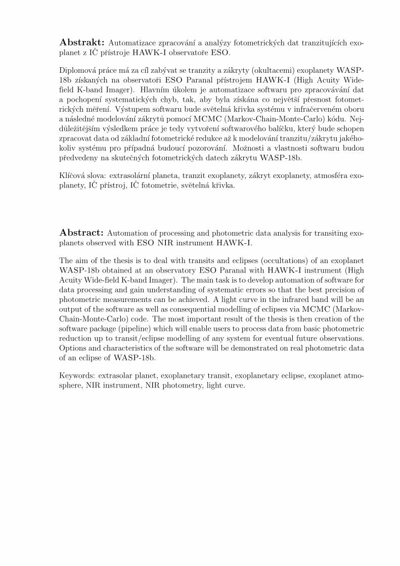
Abstrakt: Automatizace zpracovanı a analyzy fotometrickych dat tranzitujıcıch exo-planet z IC prıstroje HAWK-I observatore ESO.

Diplomova prace ma za cıl zabyvat se tranzity a zakryty (okultacemi) exoplanety WASP-18b zıskanych na observatori ESO Paranal prıstrojem HAWK-I (High Acuity Wide-field K-band Imager). Hlavnım ukolem je automatizace softwaru pro zpracovavanı data pochopenı systematickych chyb, tak, aby byla zıskana co nejvetsı presnost fotomet-rickych merenı. Vystupem softwaru bude svetelna krivka systemu v infracervenem oborua nasledne modelovanı zakrytu pomocı MCMC (Markov-Chain-Monte-Carlo) kodu. Nej-dulezitejsım vysledkem prace je tedy vytvorenı softwaroveho balıcku, ktery bude schopenzpracovat data od zakladnı fotometricke redukce az k modelovanı tranzitu/zakrytu jakeho-koliv systemu pro prıpadna budoucı pozorovanı. Moznosti a vlastnosti softwaru budoupredvedeny na skutecnych fotometrickych datech zakrytu WASP-18b.

Klıcova slova: extrasolarnı planeta, tranzit exoplanety, zakryt exoplanety, atmosfera exo-planety, IC prıstroj, IC fotometrie, svetelna krivka.

Abstract: Automation of processing and photometric data analysis for transiting exo-planets observed with ESO NIR instrument HAWK-I.

The aim of the thesis is to deal with transits and eclipses (occultations) of an exoplanetWASP-18b obtained at an observatory ESO Paranal with HAWK-I instrument (HighAcuity Wide-field K-band Imager). The main task is to develop automation of software fordata processing and gain understanding of systematic errors so that the best precision ofphotometric measurements can be achieved. A light curve in the infrared band will be anoutput of the software as well as consequential modelling of eclipses via MCMC (Markov-Chain-Monte-Carlo) code. The most important result of the thesis is then creation of thesoftware package (pipeline) which will enable users to process data from basic photometricreduction up to transit/eclipse modelling of any system for eventual future observations.Options and characteristics of the software will be demonstrated on real photometric dataof an eclipse of WASP-18b.

Keywords: extrasolar planet, exoplanetary transit, exoplanetary eclipse, exoplanet atmo-sphere, NIR instrument, NIR photometry, light curve.

Acknowledgement

I would like to thank to my supervisor Dr. Petr Kabath (Astronomical Institute, Academyof Sciences, Ondrejov), consultant Mgr. Tereza Klocova, Ph.D. (Astronomical Institute,Academy of Sciences, Ondrejov), and to Mgr. Tereza Jerabkova (Charles University,Prague) and Dipl.-Phys. Felix Rucker (Technical University of Munich) for their helpwith Python.

I declare that this thesis was written by my own with the use of cited resources.

Brno January 5th, 2017 ........................................Martin Blazek

There’s a dark but there’s a light,there could be who do not fight.

it is long time and it is far,we don’t still know which is Their star.

But who wants to see, who wants to know,he upheaves his eyes and searches slow.

On this journey there’s not the only cliff,yet it’s worth for those who say “What if”.

THE AUTHOR

Contents

1. Introduction 111.1. History . . . . . . . . . . . . . . . . . . . . . . . . . . . . . . . . . . . . . . 121.2. WASP-18 . . . . . . . . . . . . . . . . . . . . . . . . . . . . . . . . . . . . 181.3. Exoplanet atmospheres . . . . . . . . . . . . . . . . . . . . . . . . . . . . . 19

1.3.1. The atmosphere of WASP-18b . . . . . . . . . . . . . . . . . . . . 19

2. Methods to detect and characterise exoplanets 212.1. Geometry of eclipses . . . . . . . . . . . . . . . . . . . . . . . . . . . . . . 22

2.1.1. Transmission spectroscopy . . . . . . . . . . . . . . . . . . . . . . . 232.1.2. Emission photometry . . . . . . . . . . . . . . . . . . . . . . . . . . 24

3. Instruments 253.1. ESO . . . . . . . . . . . . . . . . . . . . . . . . . . . . . . . . . . . . . . . 253.2. Near-Infrared Instruments . . . . . . . . . . . . . . . . . . . . . . . . . . . 253.3. High Acuity Wide-field K-band Imager—HAWK-I . . . . . . . . . . . . . . 263.4. Fast Photometry Mode . . . . . . . . . . . . . . . . . . . . . . . . . . . . . 28

4. The data set 304.1. The header . . . . . . . . . . . . . . . . . . . . . . . . . . . . . . . . . . . 314.2. Airmass during observations . . . . . . . . . . . . . . . . . . . . . . . . . . 324.3. Seeing during observations . . . . . . . . . . . . . . . . . . . . . . . . . . . 324.4. Positions of stars on a chip . . . . . . . . . . . . . . . . . . . . . . . . . . . 344.5. Reduction frames . . . . . . . . . . . . . . . . . . . . . . . . . . . . . . . . 36

4.5.1. Dark frames . . . . . . . . . . . . . . . . . . . . . . . . . . . . . . . 364.5.2. Flat-field frames . . . . . . . . . . . . . . . . . . . . . . . . . . . . 37

5. Data reduction 395.1. Developed pipeline . . . . . . . . . . . . . . . . . . . . . . . . . . . . . . . 39

5.1.1. The script pipeline.py . . . . . . . . . . . . . . . . . . . . . . . . 395.2. Dark frames . . . . . . . . . . . . . . . . . . . . . . . . . . . . . . . . . . . 40

5.2.1. Dark current measurement . . . . . . . . . . . . . . . . . . . . . . . 405.2.2. The script darks.py . . . . . . . . . . . . . . . . . . . . . . . . . . 415.2.3. The script darksStat.py . . . . . . . . . . . . . . . . . . . . . . . 42

5.3. Flat-field frames . . . . . . . . . . . . . . . . . . . . . . . . . . . . . . . . . 435.3.1. Scripts flats.py and flatsD.py . . . . . . . . . . . . . . . . . . . 445.3.2. The script flatsStat.py . . . . . . . . . . . . . . . . . . . . . . . 44

5.4. Images before and after reduction compared . . . . . . . . . . . . . . . . . 455.4.1. Scripts reductFlats.py and reductFlatsDarks.py . . . . . . . . . 47

5.5. Bad pixel mask . . . . . . . . . . . . . . . . . . . . . . . . . . . . . . . . . 49

6. Data processing 516.1. Aperture photometry . . . . . . . . . . . . . . . . . . . . . . . . . . . . . . 51

6.1.1. The script photometry.py . . . . . . . . . . . . . . . . . . . . . . . 526.2. Apertures . . . . . . . . . . . . . . . . . . . . . . . . . . . . . . . . . . . . 53

6.2.1. The script aperts.py . . . . . . . . . . . . . . . . . . . . . . . . . 546.3. Light curve . . . . . . . . . . . . . . . . . . . . . . . . . . . . . . . . . . . 54

6.3.1. The script lightCurve.py . . . . . . . . . . . . . . . . . . . . . . . 576.4. Standard deviation . . . . . . . . . . . . . . . . . . . . . . . . . . . . . . . 58

6.4.1. The script std.py . . . . . . . . . . . . . . . . . . . . . . . . . . . 60

9

6.5. Fitting . . . . . . . . . . . . . . . . . . . . . . . . . . . . . . . . . . . . . . 616.6. Discussion of the atmosphere of WASP-18b . . . . . . . . . . . . . . . . . 65

7. Conclusion 67

Bibliography 68

Internet sources 70

Appendix—Pipeline description 71

10

1. Introduction

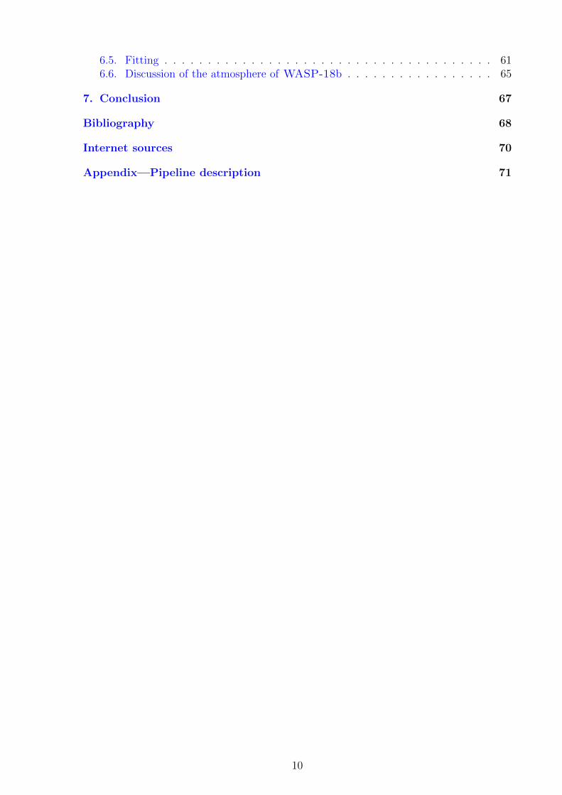
There are still a lot of people who believe that we, mankind, are alone in the Universeand that the Earth is the only planet in the Universe where a life exists. Yes, we havenot so far got any proof that the truth is different. However, there are people, especiallyscientists, who are searching for those proofs because they simply do not think that a lifeis connected strictly with the Earth. Another reason for doing that can be the attitudethat they do not want to be limited just to the Earth. It is only a tiny dot in the Sun’snearest surroundings, let alone about its importance in the Galaxy and the whole vastUniverse [figure 1].

Recently there has been a rapid progress in an exoplanetary field of astronomy andastrophysics. While relatively recently anyone hardly thought about planets beyond thesolar system, in the last few decades we discovered about two thousand extrasolar planetsand studied their physical characteristics. Moreover, it is even possible to detect theiratmospheres and explore their composition and physical processes inside them.

With this progress new questions have emerged, or in other words, the questions ofsci-fi have become fundamental ones of this field of astronomy. We can also look at thisissue from opposite side. Exoplanetary research started because scientists and peoplegenerally had begun to ask those particular questions like following:

• Is there a life in the Universe?• Is our solar system a unique one in the Galaxy (Universe)?• How does an evolution of planetary systems take place?• What are environments of planetary systems like?•What about a statistical distribution of planetary systems in the Galaxy (Universe)?

Any answer to these and related questions is neither simple nor direct but definitelyit is worth dealing with that. And searching for answers to these questions is the rightmotivation for me to write my master thesis devoted to this topic.

Figure 1: Original (from left) and zoomed images of the Earth taken by Voyager 1 fromthe distance about 6 billion kilometres. Taken from (E0).

This thesis is divided into seven chapters. The introductory chapter is devoted tohistory of exoplanets. Chapter two describes detection methods. It also includes exoplan-etary atmospheres, especially what we can find out about them currently. Near-infrared

11

instrument HAWK-I of ESO and its fast observation mode is presented in chapter three.The processed data set description, observation conditions and basic information aboutreduction frames are involved in chapter four. The fifth chapter describes data reductionand shows some statistics while the sixth chapter describes the very data processing in-cluding the obtained results. The last, seventh chapter, analyses and discusses results andwhole the process of my research and concludes the whole thesis. The appendix presentsthe decription of a developed pipeline.

1.1. History

If we look closer into the history of discovery of exoplanets, we can start with Epicurus(more than 2000 years ago) and his statement:“There are infinite worlds both like andunlike this world of ours.” He believed that there were living creatures and plants in allworlds. In the 13th century another philosopher Albertus Magnus asked a question tohimself if our world is the only one or if there are more worlds. Giordano Bruno was veryoptimistic about this problem as he asserted following (1584):“There are countless Sunsand countless Earths all rotating around their Suns in exactly the same way as the sevenplanets of our system ... The countless worlds in the Universe are no worse and no lessinhabited than our Earth.” In Newton’s age Christopher Huygens even believed (in hisbook “Cosmotheoros”—Huygens (1698)) that people on similar planets to the Earth hadastronomy and other arts (Seager, 2010).

Searching for exoplanets began with an expansion of astrometry between the first andthe second half of nineteenth century. The target was a binary system 70 Ophiuchi (thiswas the first published claim of a planet beyond our solar system—Jacob, 1855 ). In the1960s a planet around Barnard’s star was announced (van de Kamp, 1963). Eventually,none of these two “planets” was confirmed as real planets. The first two real exoplanets,announced in 1992, were orbiting a pulsar—PSR 1257+12 (Wolszczan and Frail, 1992).However, since they are supposed to be dead worlds due to a deadly radiation from theirhost star, the exoplanet research is focused on Sun-like stars.

At last, first announcement about an exoplanet around solar type star came in 1995.The planet discovered by radial velocity method has got a mass of a 0.5 MJ (Jupiter mass)and of an orbital period of 4.2 days. Its host star is a Sun-like star—51 Peg (Mayor andQueloz, 1995). That is the reason why the word “valid” is used—Sun-like stars can hostplanets with a life as we know it from the Earth in contrast to probably “dead worlds”orbiting pulsars. Discovery of this planet may be the most important discovery connectedwith exoplanets. The reason is that this planet has changed our view on planet formationand evolution theories. Giant planets have never been expected to be so close to theirparent star as this one is (seven times closer to the Sun than Mercury). These planetsare called hot Jupiters because of their size (similar to Jupiter planet of our solar system)and high temperature caused by the short distance to their star.

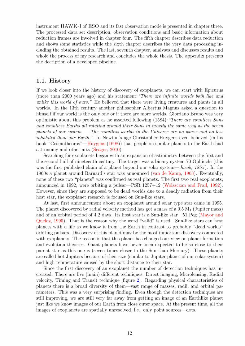
Since the first discovery of an exoplanet the number of detection techniques has in-creased. There are five (main) different techniques: Direct imaging, Microlensing, Radialvelocity, Timing and Transit technique [figure 2]. Regarding physical characteristics ofplanets there is a broad diversity of them—vast range of masses, radii, and orbital pa-rameters. This was a very surprising finding. Even though the detection techniques arestill improving, we are still very far away from getting an image of an Earthlike planetjust like we know images of our Earth from close outer space. At the present time, all theimages of exoplanets are spatially unresolved, i.e., only point sources—dots.

12

But what is actually a planet? According to the definition of the International Astro-nomical Union (IAU) established by astronomers in 2006, a planet in the Solar Systemis:

“A celestial body thata) is in orbit around the Sun,b) has sufficient mass for its self-gravity to overcome rigid body forces so that itassumes a hydrostatic equilibrium (nearly round) shape, andc) has cleared the neighbourhood around its orbit” (E1).

Another (working) definition has been established by Working Group on ExtrasolarPlanets of the IAU. The definition reads as follows (Boss et al., 2007):

“Objects with true masses below the limiting mass for thermonuclear fusion of deu-terium (currently calculated to be 13 MJ for objects of solar metallicity) that orbit starsor stellar remnants are ‘planets’ (no matter how they formed). The minimum mass/sizerequired for an extrasolar object to be considered a planet should be the same as that usedin our solar system.”

Although there are no official definitions for an exoplanet, some commonly accepteddefinitions exist. They include a few categories of exoplanets such as Giant planet, Ter-restrial planet, Habitable planet, Earth-like planet and so on. Till today there are 3545confirmed exoplanets in 2659 planetary systems and 598 multiple planet systems1 (E2).

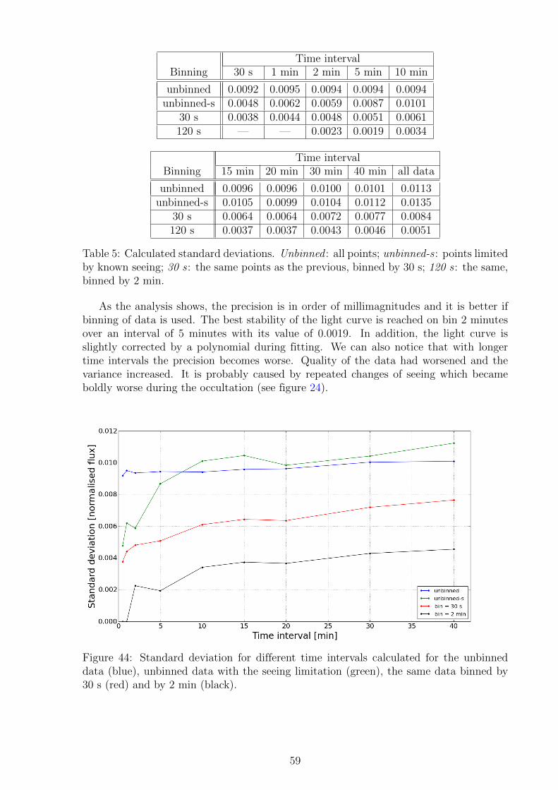
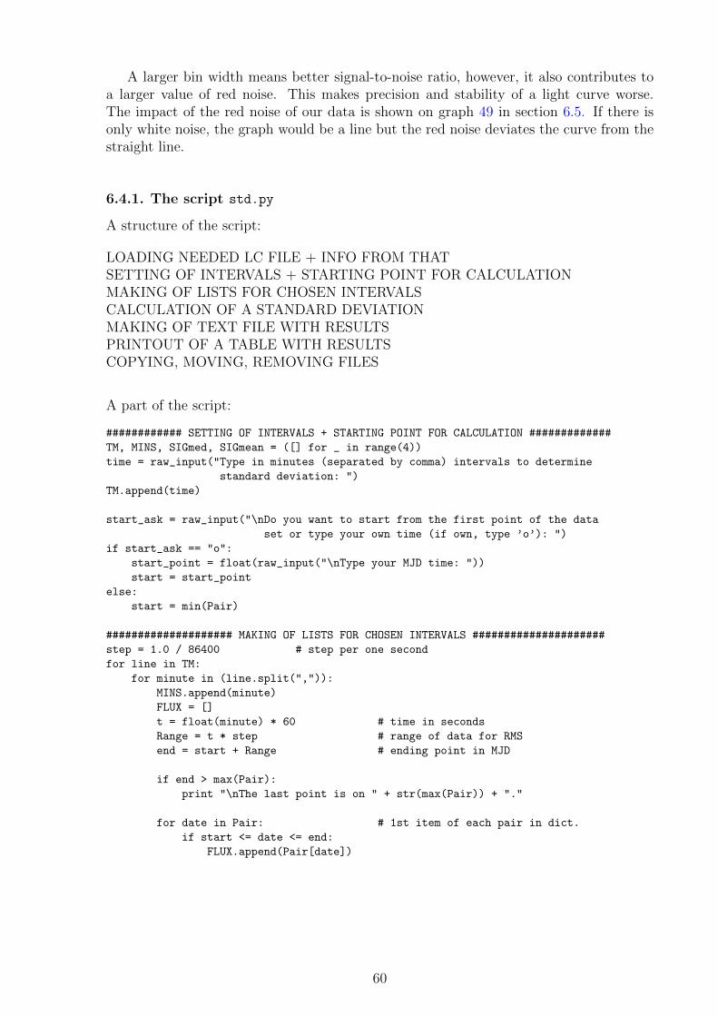
Figure 2: Number of confirmed exoplanets per year according to detection methods(17 November 2016). Taken from (E14).

111 December 2016

13

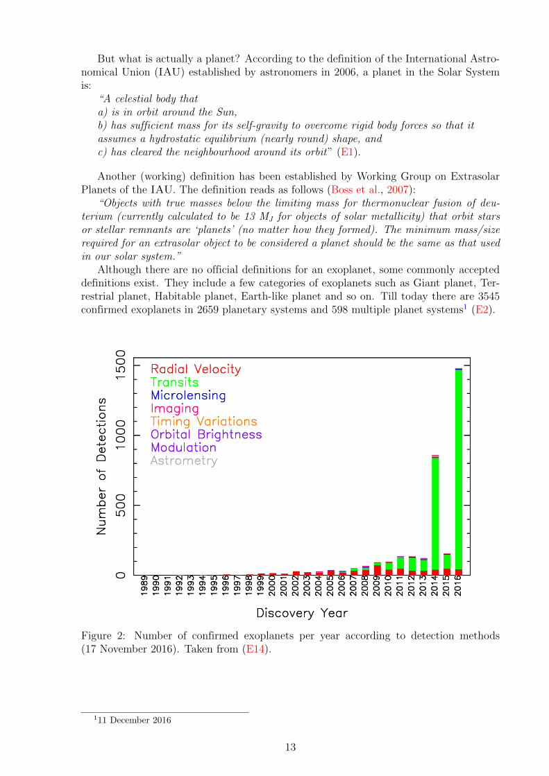
Figure 3: Kepler planet candidates divided into groups according to their sizes(23 July 2015). Taken from (E8).

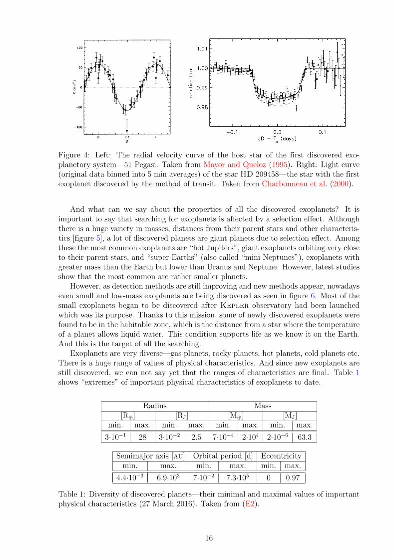
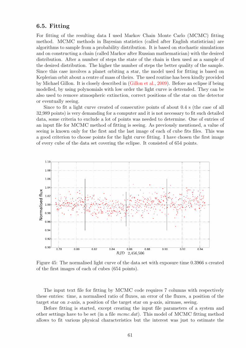
As previously mentioned, the first exoplanet has been discovered by the radial velocitymethod [figure 4 on the left]. This method is based on the fact that a star orbits the star-planet common centre of mass. The motion of a star is described by a few components.One of them is the radial velocity of the star’s motion which means the motion towards anobserver’s line-of-sight. The advantage of this technique is a possibility to detect planetswith relatively low masses. However, it has got some disadvantages. The main one isa limitation connected with a determination of an exoplanet’s mass. What we can get isa product of Mp sin i (Mp is the planet mass and i is the inclination of the orbit). Sincewe do not know the inclination angle, we can determine only the minimum mass of theexoplanet. The number of exoplanets discovered by radial velocity technique is almost500 (E3).

The unknown inclination angle can be determined by a transit method (also calledprimary eclipse). A transit occurs when, seen from the Earth, a planet passes in front ofa star. During this event the planet blocks a certain amount of light of the star and atthat moment we can detect a brightness drop which is a typical sign of a planetary transit.This drop of light then can be seen in a light curve (LC)—dependency of a radiation fluxon time. To detect a transit, the star-exoplanet plane of orbit has to be aligned with theplane of an observer’s sight. The bigger radius of a star and smaller semimajor axis ofa planet orbiting the star, the higher the probability of a transit. Small semimajor axismeans short period of the orbit of a planet and it implies a fact that by a transit methodwe detect mainly short-period exoplanets. From transits we can obtain information whichcan not be obtained by radial velocity technique. The first exoplanet discovered by thetransit method was confirmed in 2000 (Charbonneau et al., 2000). The planet is namedHD 209458b [figure 4 on the right]. Till today about 1300 exoplanets have been discoveredby the transit method (E2).

Since the number of methods had been increasing and new exoplanets had still beendiscovered, various space missions and ground based projects were launched. The mostimportant are the following:

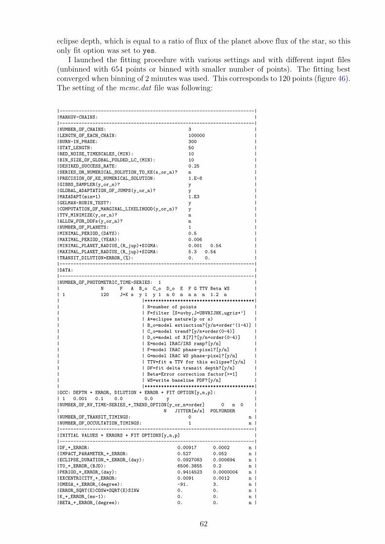
14

•CoRoTCoRoTCoRoTCoRoTCoRoTCoRoT (COnvection ROtation and planetary Transits)—French space miss-ion aimed at searching for exoplanets of a terrestrial size and at detecting astroseismo-logy. It was working between 2007 and 2013 and found about 25 exoplanets (E4).•Gaia—Space observatory of the European Space Agency (ESA) which was launched

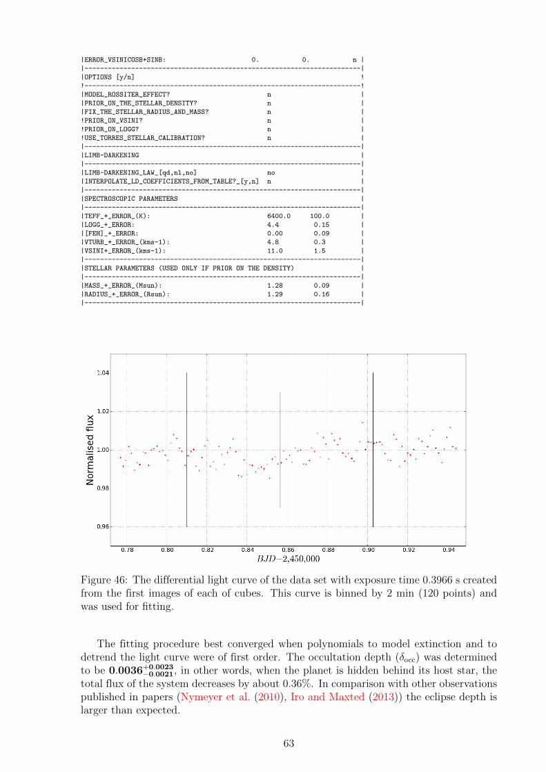
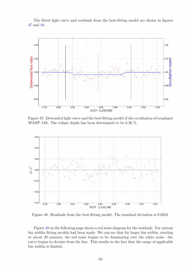
at the end of 2013 and which is planned to work until 2019. By using astrometryand transit method it should discover exoplanets of higher masses, however, due toa technical problem on Gaia it has not discovered any exoplanet yet (E5).• HAT (Hungarian-made Automated Telescope Network)—network of six te-

lescopes. The goal of the project was to find variable stars and to detect exoplanetsusing the transit method. This project operated from 1999 to 2001 and discoveredabout 60 exoplanets (E6). Since 2009 HAT-South (HATS) had joined this projectand discovered almost 20 exoplanets till today (E7).•KeplerKeplerKeplerKeplerKeplerKeplerKeplerKeplerKeplerKeplerKeplerKeplerKeplerKeplerKeplerKeplerKepler—NASA space observatory launched in 2009. It is aimed at searching

for Earth-like planets nearby habitable zone. Kepler’s photometer continually mon-itors thousands of main sequence stars and for sequential processing on the Earththe transit method is used. Today there are 2330 confirmed exoplanets and 4706candidates2 [figure 3] (E8).• K2 (“Second Light”)—Due to certain failures of Kepler’s spacecraft K2 compen-

sated for Kepler mission. For a planet searching K2 uses a method of transit andgravitational microlensing. It is planned to work until 2018 and till today it hasdiscovered over 170 exoplanets and over 450 are planet candidates (E9).• OGLE (Optical Gravitational Lensing Experiment)—Polish project, mainly

aimed at discovering dark matter, uses microlensing technique. The project itselfhad begun in 1992 but only starting the third phase in 2001 discoveries of exoplanetsbegan. It discovered more than 30 exoplanets till today (E10).•WASP (Wide Angle Search for Planets)—An international project, which be-

gan in 1999, uses the method of transit photometry. It found its first exoplanet in2006 and till today the number of discovered exoplanets by WASP is more than 130exoplanets (E11).

Currently there are some research projects being planned whose purpose is (amongothers) exoplanet research. The most important ones are following:

•E-ELT (European Extremely Large Telescope)—It will be the largest telescopeof the world, working at optical/near-infrared band. It is now under constructionon Cerro Armazones mountain in Chile by the European Southern Observatory.Its first light is planned for the year 2024. Apart from other scientific goals E-ELTwill search for exoplanets, including the planets whose mass is lower than the massof the Earth, image Earh-like planets, show Jupiter-like planets details and alsostudy atmospheres of exoplanets (E12).• JWST (James Webb Space Telescope)—Space observatory with the largest

infrared telescope, operated by ESA, Canadian Space Agency (CSA), and NationalAeronautics and Space Administration (NASA). It is now under construction andplanned to be launched in October of 2018. One of main aims of JWST is to studyexoplanets by using transit method, atmospheres of exoplanets by spectroscopymethod and direct imaging of exoplanets (E13).

211 December 2016 (E8).

15

Figure 4: Left: The radial velocity curve of the host star of the first discovered exo-planetary system—51 Pegasi. Taken from Mayor and Queloz (1995). Right: Light curve(original data binned into 5 min averages) of the star HD 209458—the star with the firstexoplanet discovered by the method of transit. Taken from Charbonneau et al. (2000).

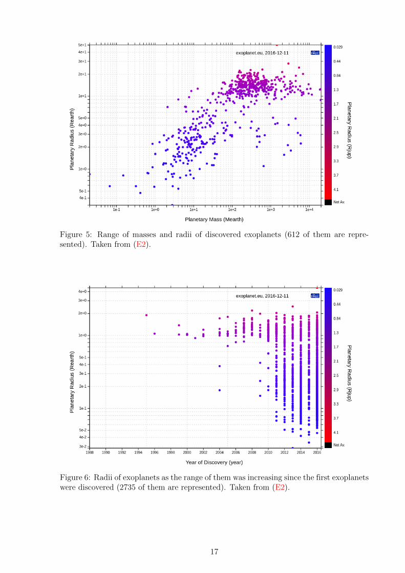
And what can we say about the properties of all the discovered exoplanets? It isimportant to say that searching for exoplanets is affected by a selection effect. Althoughthere is a huge variety in masses, distances from their parent stars and other characteris-tics [figure 5], a lot of discovered planets are giant planets due to selection effect. Amongthese the most common exoplanets are “hot Jupiters”, giant exoplanets orbiting very closeto their parent stars, and “super-Earths” (also called “mini-Neptunes”), exoplanets withgreater mass than the Earth but lower than Uranus and Neptune. However, latest studiesshow that the most common are rather smaller planets.

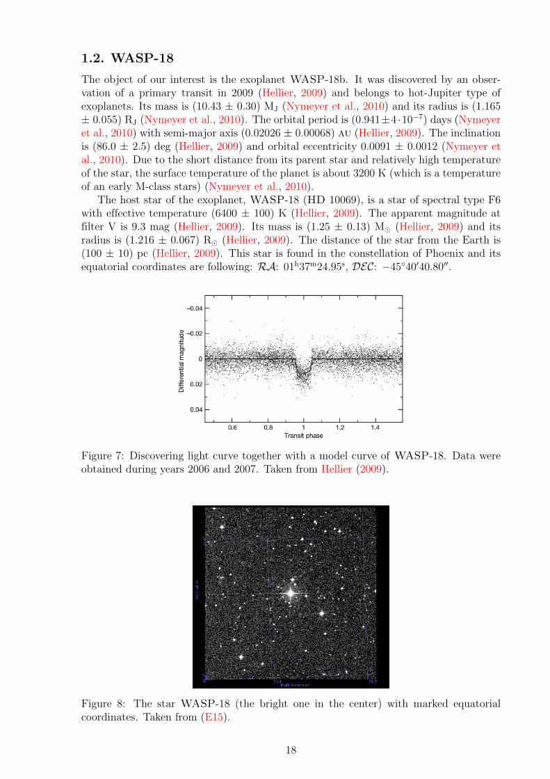
However, as detection methods are still improving and new methods appear, nowadayseven small and low-mass exoplanets are being discovered as seen in figure 6. Most of thesmall exoplanets began to be discovered after Kepler observatory had been launchedwhich was its purpose. Thanks to this mission, some of newly discovered exoplanets werefound to be in the habitable zone, which is the distance from a star where the temperatureof a planet allows liquid water. This condition supports life as we know it on the Earth.And this is the target of all the searching.

Exoplanets are very diverse—gas planets, rocky planets, hot planets, cold planets etc.There is a huge range of values of physical characteristics. And since new exoplanets arestill discovered, we can not say yet that the ranges of characteristics are final. Table 1shows “extremes” of important physical characteristics of exoplanets to date.

Radius Mass[R⊕] [RJ] [M⊕] [MJ]

min. max. min. max. min. max. min. max.

3·10−1 28 3·10−2 2.5 7·10−4 2·104 2·10−6 63.3

Semimajor axis [au] Orbital period [d] Eccentricitymin. max. min. max. min. max.

4.4·10−3 6.9·103 7·10−2 7.3·105 0 0.97

Table 1: Diversity of discovered planets—their minimal and maximal values of importantphysical characteristics (27 March 2016). Taken from (E2).

16

Figure 5: Range of masses and radii of discovered exoplanets (612 of them are repre-sented). Taken from (E2).

Figure 6: Radii of exoplanets as the range of them was increasing since the first exoplanetswere discovered (2735 of them are represented). Taken from (E2).

17

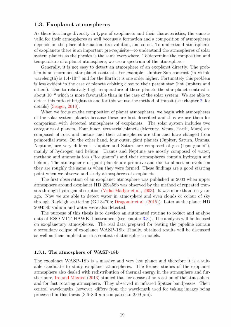
1.2. WASP-18

The object of our interest is the exoplanet WASP-18b. It was discovered by an obser-vation of a primary transit in 2009 (Hellier, 2009) and belongs to hot-Jupiter type ofexoplanets. Its mass is (10.43 ± 0.30) MJ (Nymeyer et al., 2010) and its radius is (1.165± 0.055) RJ (Nymeyer et al., 2010). The orbital period is (0.941±4 ·10−7) days (Nymeyeret al., 2010) with semi-major axis (0.02026 ± 0.00068) au (Hellier, 2009). The inclinationis (86.0 ± 2.5) deg (Hellier, 2009) and orbital eccentricity 0.0091 ± 0.0012 (Nymeyer etal., 2010). Due to the short distance from its parent star and relatively high temperatureof the star, the surface temperature of the planet is about 3200 K (which is a temperatureof an early M-class stars) (Nymeyer et al., 2010).

The host star of the exoplanet, WASP-18 (HD 10069), is a star of spectral type F6with effective temperature (6400 ± 100) K (Hellier, 2009). The apparent magnitude atfilter V is 9.3 mag (Hellier, 2009). Its mass is (1.25 ± 0.13) M� (Hellier, 2009) and itsradius is (1.216 ± 0.067) R� (Hellier, 2009). The distance of the star from the Earth is(100 ± 10) pc (Hellier, 2009). This star is found in the constellation of Phoenix and itsequatorial coordinates are following: RA: 01h37m24.95s, DEC: −45◦40′40.80′′.

Figure 7: Discovering light curve together with a model curve of WASP-18. Data wereobtained during years 2006 and 2007. Taken from Hellier (2009).

Figure 8: The star WASP-18 (the bright one in the center) with marked equatorialcoordinates. Taken from (E15).

18

1.3. Exoplanet atmospheres

As there is a large diversity in types of exoplanets and their characteristics, the same isvalid for their atmospheres as well because a formation and a composition of atmospheresdepends on the place of formation, its evolution, and so on. To understand atmospheresof exoplanets there is an important pre-requisite—to understand the atmospheres of solarsystem planets as the physics is the same everywhere. To determine the composition andtemperature of a planet atmosphere, we use a spectrum of the atmosphere.

Generally, it is not easy to detect an atmosphere of an exoplanet directly. The prob-lem is an enormous star-planet contrast. For example—Jupiter-Sun contrast (in visiblewavelength) is 1.4 ·10−9 and for the Earth it is one order higher. Fortunately this problemis less evident in the case of planets orbiting close to their parent star (hot Jupiters andothers). Due to relatively high temperature of these planets the star-planet contrast isabout 10−3 which is more favourable than in the case of the solar system. We are able todetect this ratio of brightness and for this we use the method of transit (see chapter 2. fordetails) (Seager, 2010).

When we focus on the composition of planet atmospheres, we begin with atmospheresof the solar system planets because these are best described and thus we use them forcomparison with detected atmospheres of exoplanets. The solar system includes twocategories of planets. Four inner, terrestrial planets (Mercury, Venus, Earth, Mars) arecomposed of rock and metals and their atmospheres are thin and have changed fromprimordial state. On the other hand, four outer, giant planets (Jupiter, Saturn, Uranus,Neptune) are very different. Jupiter and Saturn are composed of gas (“gas giants”),mainly of hydrogen and helium. Uranus and Neptune are mostly composed of water,methane and ammonia ices (“ice giants”) and their atmospheres contain hydrogen andhelium. The atmospheres of giant planets are primitive and due to almost no evolutionthey are roughly the same as when they were formed. These findings are a good startingpoint when we observe and study atmospheres of exoplanets.

The first observation of an exoplanet atmosphere was published in 2003 when upperatmosphere around exoplanet HD 209458b was observed by the method of repeated tran-sits through hydrogen absorption (Vidal-Madjar et al., 2003). It was more than ten yearsago. Now we are able to detect water in atmosphere and even clouds or colour of skythrough Rayleigh scattering (GJ 3470b; Dragomir et al. (2015)). Later at the planet HD209458b sodium and water were also detected.

The purpose of this thesis is to develop an automated routine to reduct and analysedata of ESO VLT HAWK-I instrument (see chapter 3.3.). The analysis will be focusedon exoplanetary atmospheres. The real data prepared for testing the pipeline containa secondary eclipse of exoplanet WASP-18b. Finally, obtained results will be discussedas well as their implication in a context of atmospheric models.

1.3.1. The atmosphere of WASP-18b

The exoplanet WASP-18b is a massive and very hot planet and therefore it is a suit-able candidate to study exoplanet atmospheres. The former studies of the exoplanetatmosphere also dealed with redistribution of thermal energy in the atmosphere and fur-thermore, Iro and Maxted (2013) studied that for a case of no rotation of the atmosphereand for fast rotating atmosphere. They observed in infrared Spitzer bandpasses. Theircentral wavelengths, however, differs from the wavelength used for taking images beingprocessed in this thesis (3.6–8.0 µm compared to 2.09 µm).

19

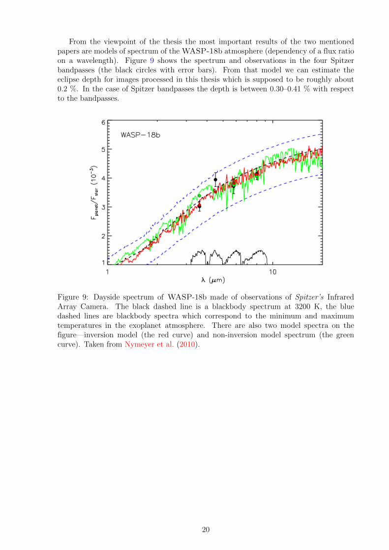
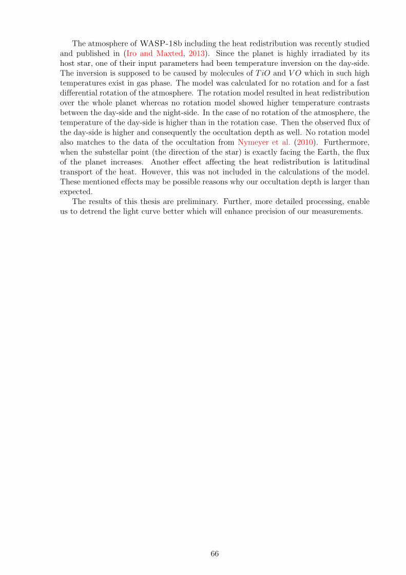
From the viewpoint of the thesis the most important results of the two mentionedpapers are models of spectrum of the WASP-18b atmosphere (dependency of a flux ratioon a wavelength). Figure 9 shows the spectrum and observations in the four Spitzerbandpasses (the black circles with error bars). From that model we can estimate theeclipse depth for images processed in this thesis which is supposed to be roughly about0.2 %. In the case of Spitzer bandpasses the depth is between 0.30–0.41 % with respectto the bandpasses.

Figure 9: Dayside spectrum of WASP-18b made of observations of Spitzer’s InfraredArray Camera. The black dashed line is a blackbody spectrum at 3200 K, the bluedashed lines are blackbody spectra which correspond to the minimum and maximumtemperatures in the exoplanet atmosphere. There are also two model spectra on thefigure—inversion model (the red curve) and non-inversion model spectrum (the greencurve). Taken from Nymeyer et al. (2010).

20

2. Methods to detect and characterise exoplanets

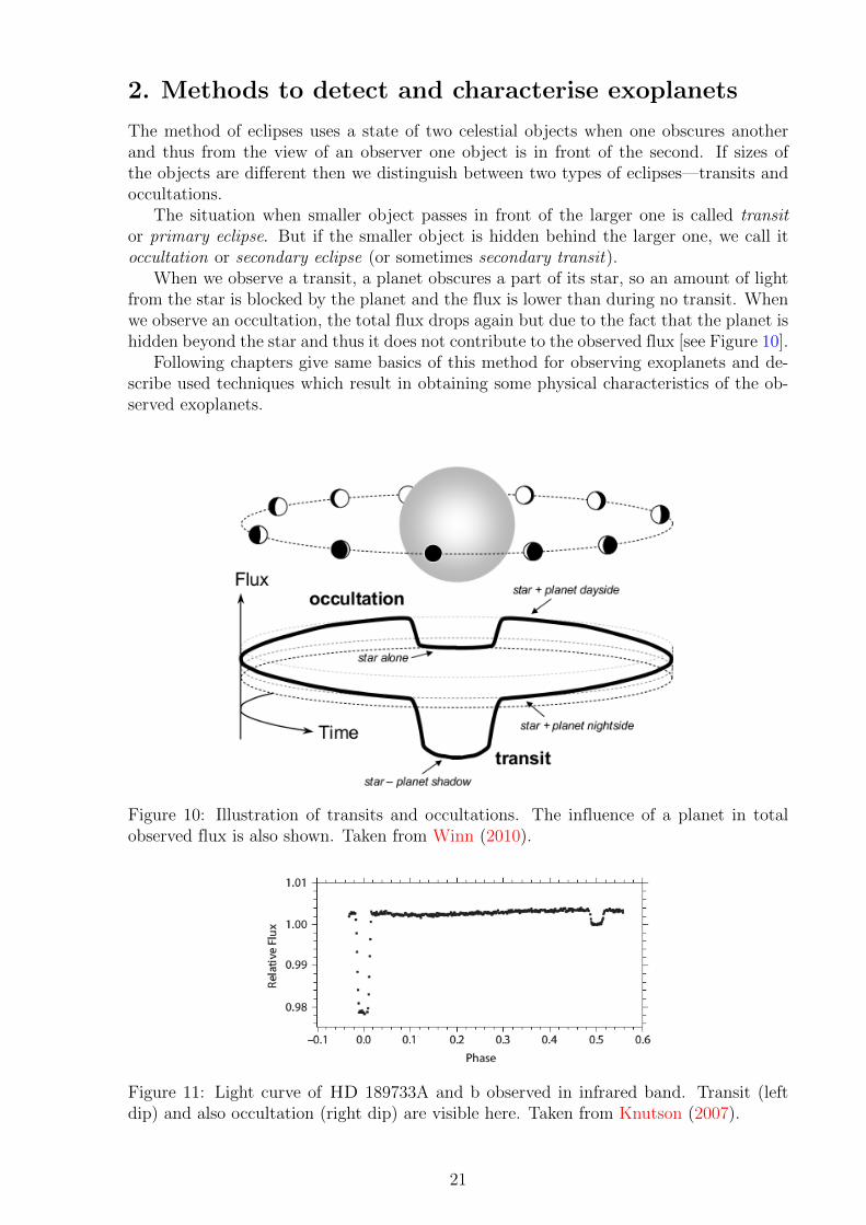
The method of eclipses uses a state of two celestial objects when one obscures anotherand thus from the view of an observer one object is in front of the second. If sizes ofthe objects are different then we distinguish between two types of eclipses—transits andoccultations.

The situation when smaller object passes in front of the larger one is called transitor primary eclipse. But if the smaller object is hidden behind the larger one, we call itoccultation or secondary eclipse (or sometimes secondary transit).

When we observe a transit, a planet obscures a part of its star, so an amount of lightfrom the star is blocked by the planet and the flux is lower than during no transit. Whenwe observe an occultation, the total flux drops again but due to the fact that the planet ishidden beyond the star and thus it does not contribute to the observed flux [see Figure 10].

Following chapters give same basics of this method for observing exoplanets and de-scribe used techniques which result in obtaining some physical characteristics of the ob-served exoplanets.

Figure 10: Illustration of transits and occultations. The influence of a planet in totalobserved flux is also shown. Taken from Winn (2010).

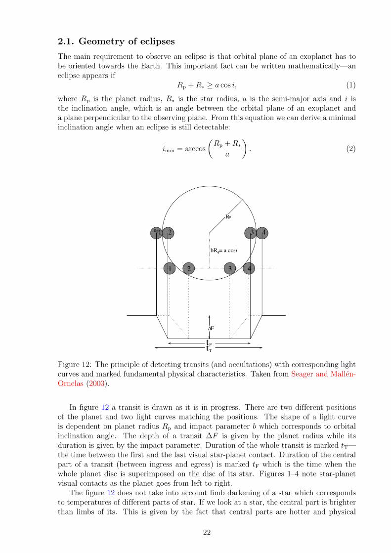
Figure 11: Light curve of HD 189733A and b observed in infrared band. Transit (leftdip) and also occultation (right dip) are visible here. Taken from Knutson (2007).

21

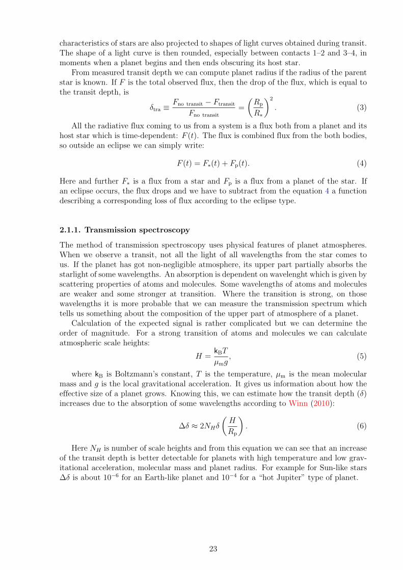
2.1. Geometry of eclipses

The main requirement to observe an eclipse is that orbital plane of an exoplanet has tobe oriented towards the Earth. This important fact can be written mathematically—aneclipse appears if

Rp +R∗ ≥ a cos i, (1)

where Rp is the planet radius, R∗ is the star radius, a is the semi-major axis and i isthe inclination angle, which is an angle between the orbital plane of an exoplanet anda plane perpendicular to the observing plane. From this equation we can derive a minimalinclination angle when an eclipse is still detectable:

imin = arccos

(Rp +R∗

a

). (2)

Figure 12: The principle of detecting transits (and occultations) with corresponding lightcurves and marked fundamental physical characteristics. Taken from Seager and Mallen-Ornelas (2003).

In figure 12 a transit is drawn as it is in progress. There are two different positionsof the planet and two light curves matching the positions. The shape of a light curveis dependent on planet radius Rp and impact parameter b which corresponds to orbitalinclination angle. The depth of a transit ∆F is given by the planet radius while itsduration is given by the impact parameter. Duration of the whole transit is marked tT—the time between the first and the last visual star-planet contact. Duration of the centralpart of a transit (between ingress and egress) is marked tF which is the time when thewhole planet disc is superimposed on the disc of its star. Figures 1–4 note star-planetvisual contacts as the planet goes from left to right.

The figure 12 does not take into account limb darkening of a star which correspondsto temperatures of different parts of star. If we look at a star, the central part is brighterthan limbs of its. This is given by the fact that central parts are hotter and physical

22

characteristics of stars are also projected to shapes of light curves obtained during transit.The shape of a light curve is then rounded, especially between contacts 1–2 and 3–4, inmoments when a planet begins and then ends obscuring its host star.

From measured transit depth we can compute planet radius if the radius of the parentstar is known. If F is the total observed flux, then the drop of the flux, which is equal tothe transit depth, is

δtra ≡Fno transit − Ftransit

Fno transit

=

(Rp

R∗

)2

. (3)

All the radiative flux coming to us from a system is a flux both from a planet and itshost star which is time-dependent: F (t). The flux is combined flux from the both bodies,so outside an eclipse we can simply write:

F (t) = F∗(t) + Fp(t). (4)

Here and further F∗ is a flux from a star and Fp is a flux from a planet of the star. Ifan eclipse occurs, the flux drops and we have to subtract from the equation 4 a functiondescribing a corresponding loss of flux according to the eclipse type.

2.1.1. Transmission spectroscopy

The method of transmission spectroscopy uses physical features of planet atmospheres.When we observe a transit, not all the light of all wavelengths from the star comes tous. If the planet has got non-negligible atmosphere, its upper part partially absorbs thestarlight of some wavelengths. An absorption is dependent on wavelenght which is given byscattering properties of atoms and molecules. Some wavelengths of atoms and moleculesare weaker and some stronger at transition. Where the transition is strong, on thosewavelengths it is more probable that we can measure the transmission spectrum whichtells us something about the composition of the upper part of atmosphere of a planet.

Calculation of the expected signal is rather complicated but we can determine theorder of magnitude. For a strong transition of atoms and molecules we can calculateatmospheric scale heights:

H =kBT

µmg, (5)

where kB is Boltzmann’s constant, T is the temperature, µm is the mean molecularmass and g is the local gravitational acceleration. It gives us information about how theeffective size of a planet grows. Knowing this, we can estimate how the transit depth (δ)increases due to the absorption of some wavelengths according to Winn (2010):

∆δ ≈ 2NHδ

(H

Rp

). (6)

Here NH is number of scale heights and from this equation we can see that an increaseof the transit depth is better detectable for planets with high temperature and low grav-itational acceleration, molecular mass and planet radius. For example for Sun-like stars∆δ is about 10−6 for an Earth-like planet and 10−4 for a “hot Jupiter” type of planet.

23

2.1.2. Emission photometry

When we observe an occultation of a planet, the depth of the occultation, measured froman obtained light curve, gives us a ratio of fluxes from a measured planet and its hoststar, so

δocc ∝Fp

F∗. (7)

During an occultation, the whole planet is hidden and flux coming to us declines. Thedepth of the occultation is dependent on intensity and radius of the planet and the star:

δocc = k2IpI∗, (8)

where k = Rp/R∗ and Ip and I∗ are averaged intensities of the disk of the planet andthe star, respectively. From the equation 8 is seen how transit and occultation depth areconnected, as k2 = (Rp/R∗)

2 (see equation 3). If we do an observation of a secondaryeclipse of an exoplanet, a transit observation has been usually done formerly and hencek is known.

There are two sources of planetary radiation—reflected light from the host star andthermal radiation from the planet itself. The thermal radiation emerges at shorterwavelengths than the reflected starlight because the planet is colder than its host star.A wavelength-dependent occultation depth can also be expressed by using the Planckfunction,

Bλ(T ) ≡ 2hc2

λ51

e(hc/λkBT ) − 1, (9)

where by approximating the both bodies as blackbody radiators

δocc(λ) = k2Bλ(Tp)

Bλ(T∗). (10)

In these equations h is the Planck’s constant, c is the speed of light, λ is the wavelengthand T is the temperature (Tp for the planet and T∗ for its star). By integrating theequation 10 over the bandpass we obtain the observed δocc.

Disks of planets are not uniformly bright and depending on a type of planet (gaseous,rocky, ...) they can have zones which can differ by brightness. By getting a light curve ofan occultation we can obtain from its ingress and egress part information how brightnessof a planet is distributed.

24

3. Instruments

3.1. ESO

The European Southern Observatory (ESO) is an astronomical organization which isone of the most important organizations of astronomic research. It was established in1962 and today it has already got 16 member countries (Austria, Belgium, Brazil, CzechRepublic, Denmark, Finland, France, Germany, Holland, Italy, Poland, Portugal, Spain,Sweden, Switzerland and United Kingdom) and Chile as the host state. The headquartersof ESO is located in Garching (near Munich) in Germany. Currently ESO operates threeobservatories: Chajnantor, La Silla and Paranal. The name of each of the observatoriescomes from the name of the mountain where the observatory is found. All of them aresituated in the Atacama desert in Chile because this area is very suitable for astronomicalobservations due to the high altitude, an excellent dry climate and a lot of clear nightsduring a year.

Chajnantor observatory lies at the altitude of 5000 m where Atacama Large Millime-ter/submillimeter Array (ALMA) is situated. It consists of 66 giant antennas.

La Silla observatory lies at the altitude of 2400 m and its equipment consists of a fewtelescopes working in the optical band. Diameters of their mirrors are up to 3.6 m.

Paranal observatory lies at the altitude of 2600 m and it is situated on one of thedriest regions in the world. There are four main telescopes which are called Very LargeTelescope (VLT). Each of them has got its primary mirror with the diameter of 8.2 m.There are also four Auxiliary Telescopes with main mirrors of 1.8 m in diameter. In anindividual use of a Unit Telescope images of celestial objects as faint as 30 mag can beobtained. VLT instrumentation includes large-field imagers, cameras and spectrographswith adaptive optics and so on. It covers a broad spectral region—from deep ultravioletto mid-infrared wavelengths. All the telescopes can work separately or together to forma giant interferometer.

Currently ESO is constructing European Extremely Large optical/infrared Telescope(E-ELT) which will have a 39-metres primary mirror. It will be the largest telescope inthe world for visible and near-infrared band and its launching is planned for 2024.

3.2. Near-Infrared Instruments

When we use infrared electromagnetic radiation (IR) in physics and especially in astro-physics, for our purposes we usually distinguish among a few bands of electromagneticradiation in dependency on a wavelength. These are roughly following: Near-Infrared(NIR): 1–5 µm; Mid-Infrared (MIR): 5–25 µm; Far-Infrared (FIR): 25–1000 µm. Asa visible light we consider wavelenghts between 0.3–1.0 µm. Commonly used Charge-Coupled Devices (CCD) work just on these wavelengths.

Although CCDs and IR detectors use the same physical principle, infrared detectorsare very different from CCDs. Since IR radiation corresponds to less energy than a vis-ible light, electrons in IR detector are excited to a conduction band with small energyabout 1 eV. This process is very sensitive to temperature as it is generally known aboutinfrared radiation. Every electron has got its energy which is proportional to kT (k isthe Boltzmann constant and T is the temperature of radiation) and thus electrons canbe thermally excited into the conduction band. This, so-called “dark current”, has to bedecreased by cooling the detector to low temperature.

The most important difference between CCDs and IR detectors is from the viewof their architecture. CCDs work as charge-transfer devices when photoelectrons are

25

collected and from a row to a row then they are read out by a transfer. But IR detectorsdo not work this way. They utilize hybrid arrays in which photodetection and readouttechnologies are separated. Each of the pixels utilizes an architecture (called “unit cell”)where each pixel has got its own readout amplifier. Another difference between the twotypes of detectors is a shutter—in contrast to CCDs, there is no shutter at IR detectors,integration is defined electronically (E16).

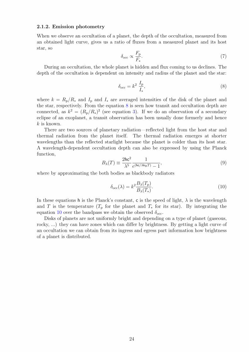
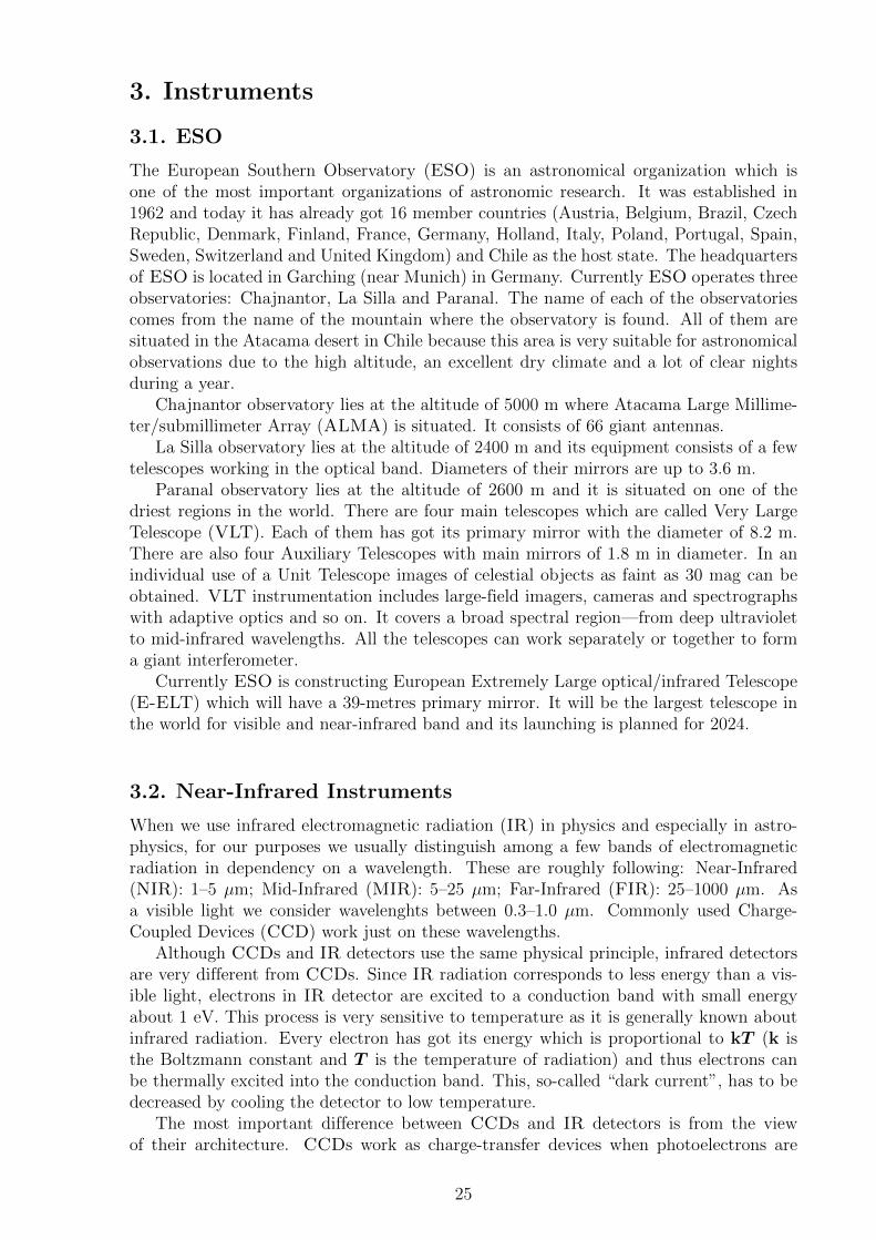
3.3. High Acuity Wide-field K-band Imager—HAWK-I

HAWK-I, mounted on VLT, is a cryogenic (120 K and detectors at 80 K) near-infrared(0.85–2.5 µm) wide-field imager. It has got a full reflective design. The light passes fourmirrors and two filter wheels before hitting a mosaic of four 2048×2048 pixel detectors.The field of view of HAWK-I on the sky is 7.5 arcmin×7.5 arcmin. The four chips areseparated by a cross-shaped gap of ∼ 15 arcsec and numbered 1–4 anti-clockwise from thebottom left as the first one. The pixel scale is 0.1064 arcsec/pix with distortions < 0.3 %across the field of view. Dark current of the instrument is around 2 electrons/pix/s andthe read-out noise is approximately 5 electrons (E12).

Figure 13: High Acuity Wide-field K-band Imager—HAWK-I. Taken from (E12).

26

Figure 14: The infrared detector of HAWK-I. Taken from (E12).

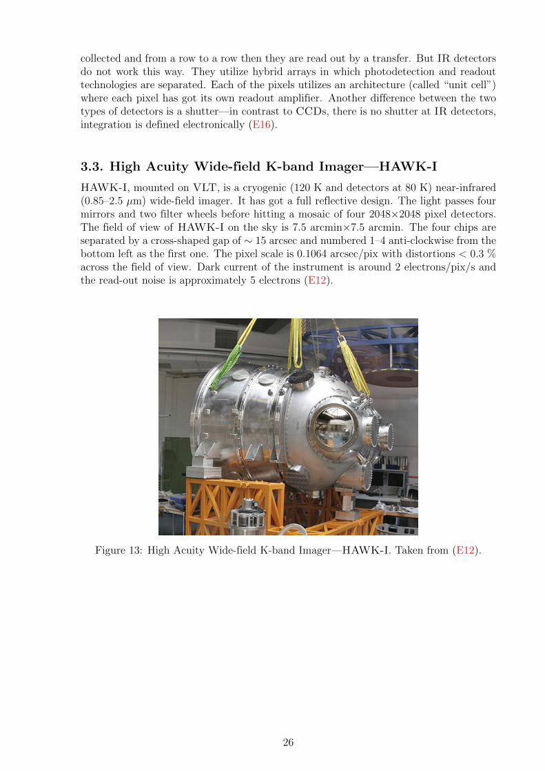
Figure 15: Raw HAWK-I dark frame, filter NB1060 (IR band), integration time 2 s.

27

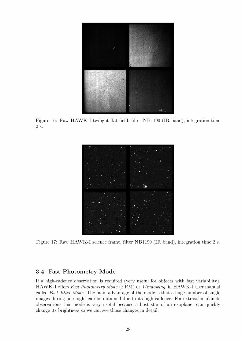
Figure 16: Raw HAWK-I twilight flat field, filter NB1190 (IR band), integration time2 s.

Figure 17: Raw HAWK-I science frame, filter NB1190 (IR band), integration time 2 s.

3.4. Fast Photometry Mode

If a high-cadence observation is required (very useful for objects with fast variability),HAWK-I offers Fast Photometry Mode (FPM) or Windowing, in HAWK-I user manualcalled Fast Jitter Mode. The main advantage of the mode is that a huge number of singleimages during one night can be obtained due to its high-cadence. For extrasolar planetsobservations this mode is very useful because a host star of an exoplanet can quicklychange its brightness so we can see those changes in detail.

28

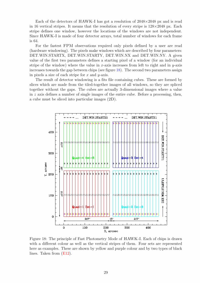
Each of the detectors of HAWK-I has got a resolution of 2048×2048 px and is readin 16 vertical stripes. It means that the resolution of every stripe is 128×2048 px. Eachstripe defines one window, however the locations of the windows are not independent.Since HAWK-I is made of four detector arrays, total number of windows for each frameis 64.

For the fastest FPM observations required only pixels defined by a user are read(hardware windowing). The pixels make windows which are described by four parameters:DET.WIN.STARTX, DET.WIN.STARTY, DET.WIN.NX and DET.WIN.NY. A givenvalue of the first two parameters defines a starting pixel of a window (for an individualstripe of the window) where the value in x-axis increases from left to right and in y-axisincreases towards the gap between chips (see figure 18). The second two parameters assignin pixels a size of each stripe for x and y-axis.

The result of detector windowing is a fits file containing cubes. These are formed byslices which are made from the tiled-together images of all windows, so they are splicedtogether without the gaps. The cubes are actually 3-dimensional images where a valuein z axis defines a number of single images of the entire cube. Before a processing, then,a cube must be sliced into particular images (2D).

Figure 18: The principle of Fast Photometry Mode of HAWK-I. Each of chips is drawnwith a different colour as well as the vertical stripes of them. Four sets are representedhere as examples. These are shown by yellow and purple colour and by two types of blacklines. Taken from (E12).

29

4. The data set

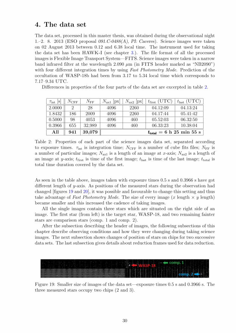
The data set, processed in this master thesis, was obtained during the observational night1.–2. 8. 2013 (ESO proposal 091.C-0488(A), PI: Caceres). Science images were takenon 02 August 2013 between 0.12 and 6.38 local time. The instrument used for takingthe data set has been HAWK-I (see chapter 3.). The file format of all the processedimages is Flexible Image Transport System—FITS. Science images were taken in a narrowband infrared filter at the wavelength 2.090 µm (in FITS header marked as “NB2090”)with four different integration times by using Fast Photometry Mode. Prediction of theoccultation of WASP-18b had been from 3.17 to 5.34 local time which corresponds to7.17–9.34 UTC.

Differences in properties of the four parts of the data set are excerpted in table 2.

τint [s] NCFF NFF Nax1 [px] Nax2 [px] tfirst (UTC) tlast (UTC)

2.0000 2 28 4096 2260 04.12:09 04.13:241.8432 186 2009 4096 2260 04.17:44 05.41:420.5000 98 4053 4096 460 05.52:03 06.32:500.3966 655 32,989 4096 460 06.33:23 10.38:04

All 941 39,079 ttotalttotalttotal = 6 h 25 min 55 s

Table 2: Properties of each part of the science images data set, separated accordingto exposure times. τint is integration time; NCFF is a number of cube fits files; NFF isa number of particular images; Nax1 is a length of an image at x-axis; Nax2 is a length ofan image at y-axis; tfirst is time of the first image; tlast is time of the last image; ttotal istotal time duration covered by the data set.

As seen in the table above, images taken with exposure times 0.5 s and 0.3966 s have gotdifferent length of y-axis. As positions of the measured stars during the observation hadchanged [figures 19 and 20], it was possible and favourable to change this setting and thustake advantage of Fast Photometry Mode. The size of every image (x length × y length)became smaller and this increased the cadence of taking images.

All the single images contain three stars which are situated on the right side of animage. The first star (from left) is the target star, WASP-18, and two remaining fainterstars are comparison stars (comp. 1 and comp. 2).

After the subsection describing the header of images, the following subsections of thischapter describe observing conditions and how they were changing during taking scienceimages. The next subsection shows changes of position of stars on chips for two successivedata sets. The last subsection gives details about reduction frames used for data reduction.

Figure 19: Smaller size of images of the data set—exposure times 0.5 s and 0.3966 s. Thethree measured stars occupy two chips (2 and 3).

30

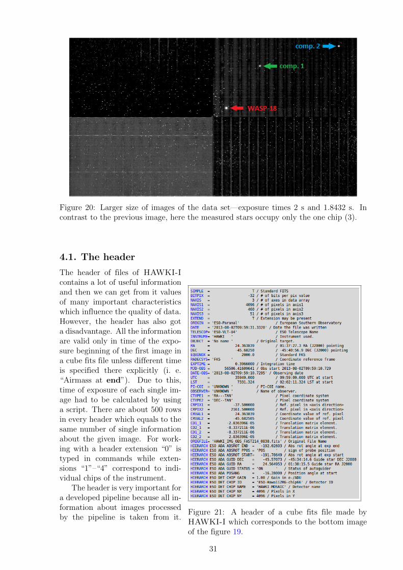
Figure 20: Larger size of images of the data set—exposure times 2 s and 1.8432 s. Incontrast to the previous image, here the measured stars occupy only the one chip (3).

4.1. The header

Figure 21: A header of a cube fits file made byHAWKI-I which corresponds to the bottom imageof the figure 19.

The header of files of HAWKI-Icontains a lot of useful informationand then we can get from it valuesof many important characteristicswhich influence the quality of data.However, the header has also gota disadvantage. All the informationare valid only in time of the expo-sure beginning of the first image ina cube fits file unless different timeis specified there explicitly (i. e.“Airmass at end”). Due to this,time of exposure of each single im-age had to be calculated by usinga script. There are about 500 rowsin every header which equals to thesame number of single informationabout the given image. For work-ing with a header extension “0” istyped in commands while exten-sions “1”–“4” correspond to indi-vidual chips of the instrument.

The header is very important fora developed pipeline because all in-formation about images processedby the pipeline is taken from it.

31

However, as the disadvantage mentioned above, observing time of each of the imageshad to be calculated.

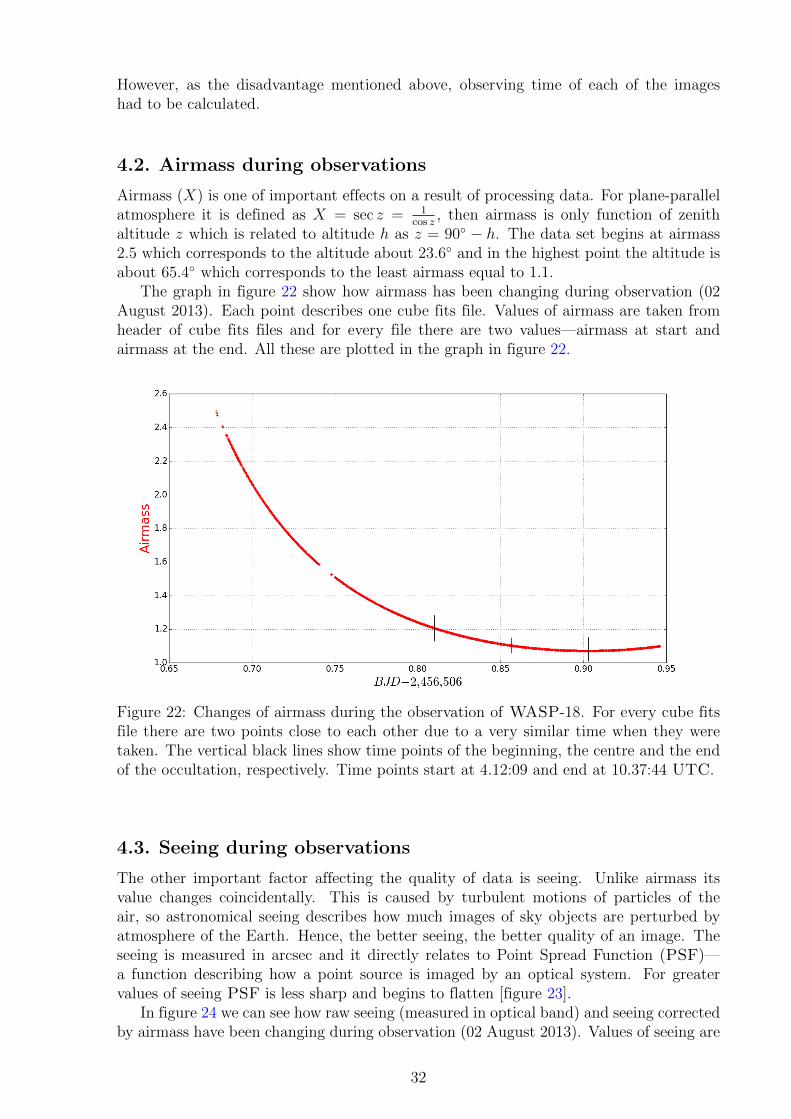
4.2. Airmass during observations

Airmass (X) is one of important effects on a result of processing data. For plane-parallelatmosphere it is defined as X = sec z = 1

cos z, then airmass is only function of zenith

altitude z which is related to altitude h as z = 90◦ − h. The data set begins at airmass2.5 which corresponds to the altitude about 23.6◦ and in the highest point the altitude isabout 65.4◦ which corresponds to the least airmass equal to 1.1.

The graph in figure 22 show how airmass has been changing during observation (02August 2013). Each point describes one cube fits file. Values of airmass are taken fromheader of cube fits files and for every file there are two values—airmass at start andairmass at the end. All these are plotted in the graph in figure 22.

Figure 22: Changes of airmass during the observation of WASP-18. For every cube fitsfile there are two points close to each other due to a very similar time when they weretaken. The vertical black lines show time points of the beginning, the centre and the endof the occultation, respectively. Time points start at 4.12:09 and end at 10.37:44 UTC.

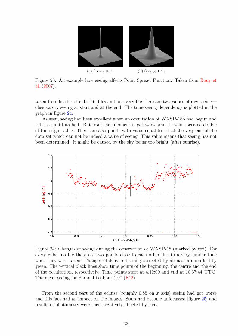
4.3. Seeing during observations

The other important factor affecting the quality of data is seeing. Unlike airmass itsvalue changes coincidentally. This is caused by turbulent motions of particles of theair, so astronomical seeing describes how much images of sky objects are perturbed byatmosphere of the Earth. Hence, the better seeing, the better quality of an image. Theseeing is measured in arcsec and it directly relates to Point Spread Function (PSF)—a function describing how a point source is imaged by an optical system. For greatervalues of seeing PSF is less sharp and begins to flatten [figure 23].

In figure 24 we can see how raw seeing (measured in optical band) and seeing correctedby airmass have been changing during observation (02 August 2013). Values of seeing are

32

(a) Seeing 0.1”. (b) Seeing 0.7”.

Figure 23: An example how seeing affects Point Spread Function. Taken from Bouy etal. (2007).

taken from header of cube fits files and for every file there are two values of raw seeing—observatory seeing at start and at the end. The time-seeing dependency is plotted in thegraph in figure 24.

As seen, seeing had been excellent when an occultation of WASP-18b had begun andit lasted until its half. But from that moment it got worse and its value became doubleof the origin value. There are also points with value equal to −1 at the very end of thedata set which can not be indeed a value of seeing. This value means that seeing has notbeen determined. It might be caused by the sky being too bright (after sunrise).

Figure 24: Changes of seeing during the observation of WASP-18 (marked by red). Forevery cube fits file there are two points close to each other due to a very similar timewhen they were taken. Changes of delivered seeing corrected by airmass are marked bygreen. The vertical black lines show time points of the beginning, the centre and the endof the occultation, respectively. Time points start at 4.12:09 and end at 10.37:44 UTC.The mean seeing for Paranal is about 1.0” (E12).

From the second part of the eclipse (roughly 0.85 on x axis) seeing had got worseand this fact had an impact on the images. Stars had become unfocussed [figure 25] andresults of photometry were then negatively affected by that.

33

(a) WASP-18. (b) Comparison star 1. (c) Comparison star 2.

Figure 25: Low quality of seeing had a negative impact on the quality of data.

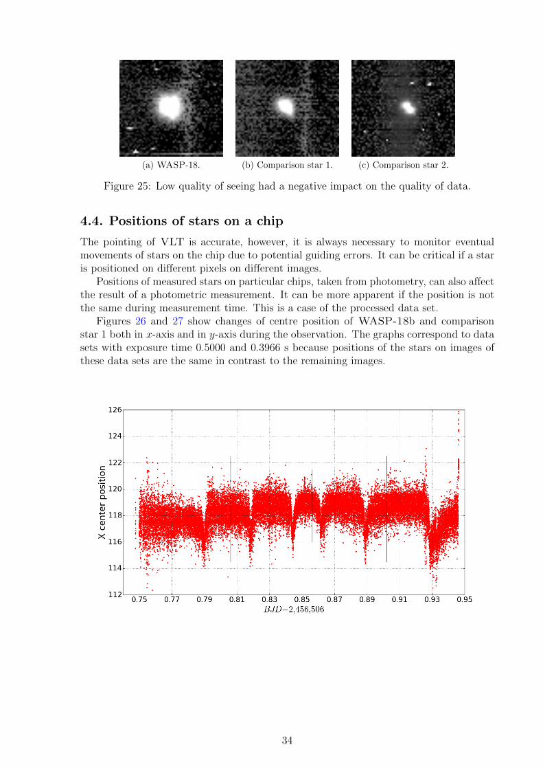
4.4. Positions of stars on a chip

The pointing of VLT is accurate, however, it is always necessary to monitor eventualmovements of stars on the chip due to potential guiding errors. It can be critical if a staris positioned on different pixels on different images.

Positions of measured stars on particular chips, taken from photometry, can also affectthe result of a photometric measurement. It can be more apparent if the position is notthe same during measurement time. This is a case of the processed data set.

Figures 26 and 27 show changes of centre position of WASP-18b and comparisonstar 1 both in x-axis and in y-axis during the observation. The graphs correspond to datasets with exposure time 0.5000 and 0.3966 s because positions of the stars on images ofthese data sets are the same in contrast to the remaining images.

34

Figure 26: Positions of stars on a chip at x-axis on images with exposure time 0.5000and 0.3966 s. The bottom graph on the previous page shows dependency on time forWASP-18b, the graph upper for comparison star 1.

From the four graphs there is obvious a small variance in the positions of the starsbut at some intervals there are “jumps” from the mean value of the position which arequickly aligned after that. These intervals are not the same, their length changes between26 and 57 minutes in x-axis and between 25 and 64 minutes in y-axis on a chip. Shiftsin the positions of the stars are about 10 pixels in the both axes while remaining on thesame chip. Due to good flat fielding this fact seems not to affect the resulting light curve.

35

Figure 27: Positions of stars on a chip at y-axis on images with exposure time 0.5000and 0.3966 s. The bottom graph on the previous page shows dependency on time forWASP-18b, the graph upper for comparison star 1.

4.5. Reduction frames

This section describes properties of dark frames and flat-field frames used for data reduc-tion. A sample of each type of a reduction frame is also shown.

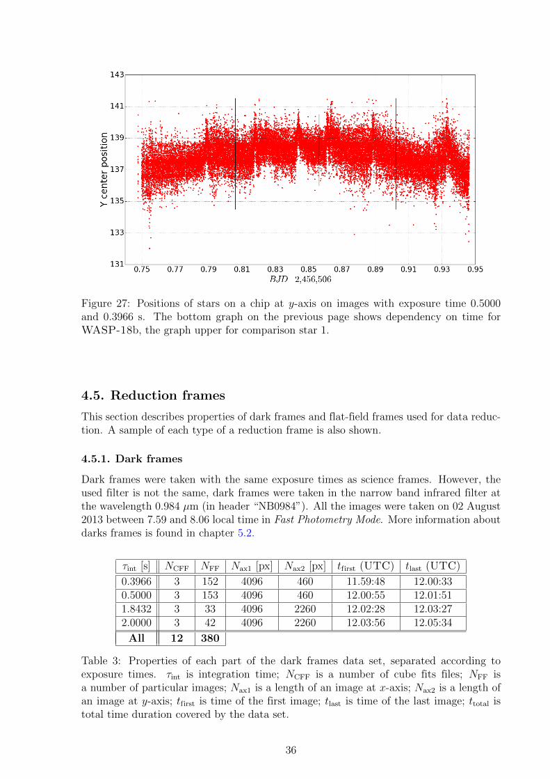
4.5.1. Dark frames

Dark frames were taken with the same exposure times as science frames. However, theused filter is not the same, dark frames were taken in the narrow band infrared filter atthe wavelength 0.984 µm (in header “NB0984”). All the images were taken on 02 August2013 between 7.59 and 8.06 local time in Fast Photometry Mode. More information aboutdarks frames is found in chapter 5.2.

τint [s] NCFF NFF Nax1 [px] Nax2 [px] tfirst (UTC) tlast (UTC)

0.3966 3 152 4096 460 11.59:48 12.00:330.5000 3 153 4096 460 12.00:55 12.01:511.8432 3 33 4096 2260 12.02:28 12.03:272.0000 3 42 4096 2260 12.03:56 12.05:34

All 12 380

Table 3: Properties of each part of the dark frames data set, separated according toexposure times. τint is integration time; NCFF is a number of cube fits files; NFF isa number of particular images; Nax1 is a length of an image at x-axis; Nax2 is a length ofan image at y-axis; tfirst is time of the first image; tlast is time of the last image; ttotal istotal time duration covered by the data set.

36

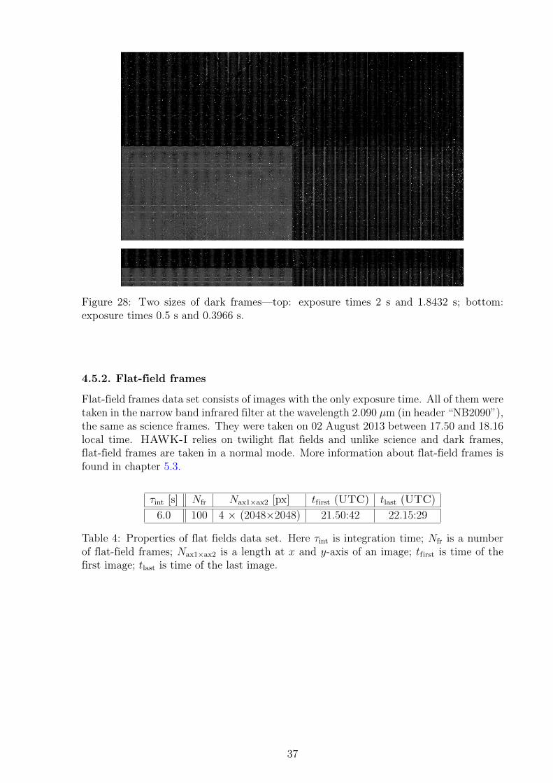
Figure 28: Two sizes of dark frames—top: exposure times 2 s and 1.8432 s; bottom:exposure times 0.5 s and 0.3966 s.

4.5.2. Flat-field frames

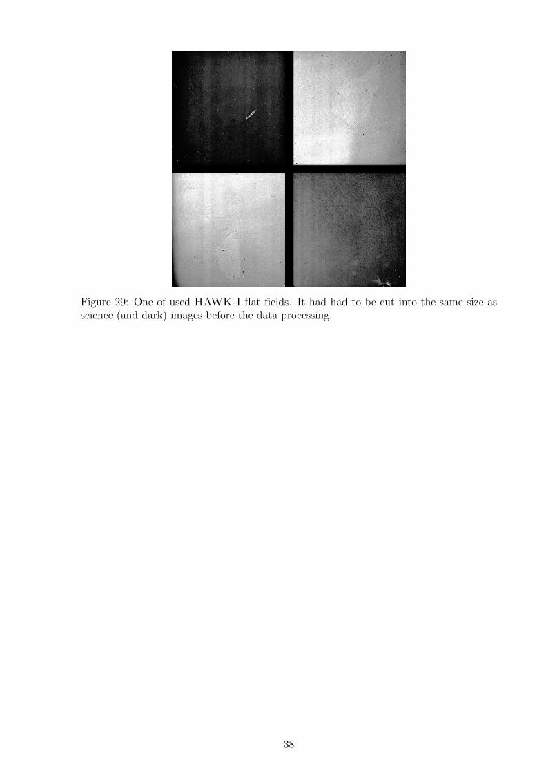
Flat-field frames data set consists of images with the only exposure time. All of them weretaken in the narrow band infrared filter at the wavelength 2.090 µm (in header “NB2090”),the same as science frames. They were taken on 02 August 2013 between 17.50 and 18.16local time. HAWK-I relies on twilight flat fields and unlike science and dark frames,flat-field frames are taken in a normal mode. More information about flat-field frames isfound in chapter 5.3.

τint [s] Nfr Nax1×ax2 [px] tfirst (UTC) tlast (UTC)

6.0 100 4 × (2048×2048) 21.50:42 22.15:29

Table 4: Properties of flat fields data set. Here τint is integration time; Nfr is a numberof flat-field frames; Nax1×ax2 is a length at x and y-axis of an image; tfirst is time of thefirst image; tlast is time of the last image.

37

Figure 29: One of used HAWK-I flat fields. It had had to be cut into the same size asscience (and dark) images before the data processing.

38

5. Data reduction

The process of data reduction is necessary to get the best results from data that we havegot. The purpose of the reduction is to remove, subtract, and correct the “instrumentsignature” introduced to a raw image by a detector. The data reduction is an instrumentspecific, however, NIR imaging follows basic rules like dark frames subtraction and flatfielding therefore a reduction process is required. To make this process easier and faster,a pipeline was developed. It will be described in following sections.

This chapter begins with introductory information about the developed pipeline. Thenext subsections give details about reduction frames including statistics. Then results ofthe data reduction are shown and discussed and the end of the chapter is devoted to a badpixel mask. Furthermore, structures and parts of Python scripts appointed for the datareduction are always appended.

5.1. Developed pipeline

The developed pipeline for HAWK-I Fast Photometry Mode consists of twelve scriptswritten in Python programming language and one configuration text file. Its goal isautomatic processing of data and the making of a light curve with basic parameters ofphotometric quantities. At the end the resulting light curve in a form of a text file isprepared for an analysis by using MCMC code.

The pipeline is started by an introductory script and after executing all commandsa next script is launched at its end. This repeats throughout the whole pipeline. Somescripts stop at a given point and require co-operation with the user.

The structure of the pipeline scripts is following:

• pipeline.py—the launching script, the option for using dark frames (N) or not (H):N darks.py—dark frames processing, the making of master dark frames;N darksStat.py (optional)—doing dark frames statistics;N flatsD.py—flat-field frames processing, the making of master flat-field frames;N flatsStat.py (optional)—doing flat-field frames statistics;N reductFlatsDarks.py—data reduction, the making of resulting images, preparing

files for photometry.

H flats.py—flat-field frames processing, the making of master flat-field frames;H flatsStat.py (optional)—doing flat-field frames statistics;H reductFlats.py—data reduction, the making of resulting images, preparing files

for photometry.• photometry.py—doing photometry;• aperts.py—choosing the best aperture for a light curve;• lightCurve.py—the making of the light curve, preparing a file for fitting routine;• std.py—determining accuracy of measurements.

5.1.1. The script pipeline.py

A structure of the script:

OPTION—WITH DARKS OR WITHOUTCLEANING THE WORKING DIRECTORY

39

GETTING INFORMATION FROM HEADER AND MAKING TEXT FILE—3D—ALLFILESMAKING OF DIRECTORIESRENAMING OF FILESGETTING INFO FROM HEADER AND MAKING TXT—3D—ALL FILES—NEWNAMESFunction—MOVING DARK FRAMES IF NOT USEDFunction—WITH DARKS OR WITHOUT

A part of the script:

#### LOADING LIBRARIES ####

from pyraf import iraf

from numpy import *

import os

from matplotlib import pylab, mlab, pyplot

###########################

########################## PARAMETERS ###############################

params = genfromtxt("config.txt", dtype = "string")

main_dir = params.take(where(params[:,0] == "main_dir")[0],0)[0,2]

flat_dir = params.take(where(params[:,0] == "flat_dir")[0],0)[0,2]

dark_dir = params.take(where(params[:,0] == "dark_dir")[0],0)[0,2]

name = params.take(where(params[:,0] == "name")[0],0)[0,2]

txt = params.take(where(params[:,0] == "txt")[0],0)[0,2]

######################## OPTION--WITH DARKS OR WITHOUT ########################

YorN = raw_input("\nDo you want to use dark frames for data reduction (’y’ or ’n’)? ")

5.2. Dark frames

Dark frames (and flat frames as well) are used to correct instrument effects influencingdata quality. However, some instruments do not require using dark frames because theirthermal noise or read-out noise is very low. This is just the case of HAWK-I (see detailsin section 3.3.).

Despite this fact, it is recommended to revise the frames, so I worked with them anddid some statistics. As HAWK-I consists of four chips, using dark frames allowed me tosee sensitivity differences among them.

To make a master dark frame I have used imcombine command and a combiningmethod median. Since not all processed images are the same size, a number of masterdark frames is corresponding to a number of sets of science images differentiated by sizes.

5.2.1. Dark current measurement

To measure a dark current of each of chips I have used all four sets of dark frames(integration times 0.3966, 0.5, 1.8432 and 2 s). By using imstat command of IRAF(Image Reduction and Analysis Facility (E17)) I had determined mean flux of each chipof all dark frames. These data then were plotted into a graph to show dependency meanflux on index.

As it is seen on the graphs below, there is linear dependency mean flux (dark current)on an integration time. Another fact is obvious from the graphs—sensitivity of all chipsis different. For the same integration time the dark current has not got the same valuefor each of the chips. The chips 1 and 2 exhibit the highest dark current, respectively.

40

100

105

110

115

120

125

130

135

140

0 20 40 60 80 100 120 140 160

Mean

ux [

counts

]

Frame number

CHIP 1:CHIP 2:CHIP 3:CHIP 4:

100

105

110

115

120

125

130

135

140

0 20 40 60 80 100 120 140 160

Mean

ux [

counts

]

Frame number


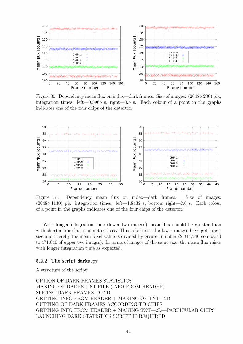
Figure 30: Dependency mean flux on index—dark frames. Size of images: (2048×230) pix,integration times: left—0.3966 s, right—0.5 s. Each colour of a point in the graphsindicates one of the four chips of the detector.

50

55

60

65

70

75

80

85

90

0 5 10 15 20 25 30 35

Mean

ux [

counts

]

Frame number


50

55

60

65

70

75

80

85

90

0 5 10 15 20 25 30 35 40 45

Mean

ux [

counts

]

Frame number


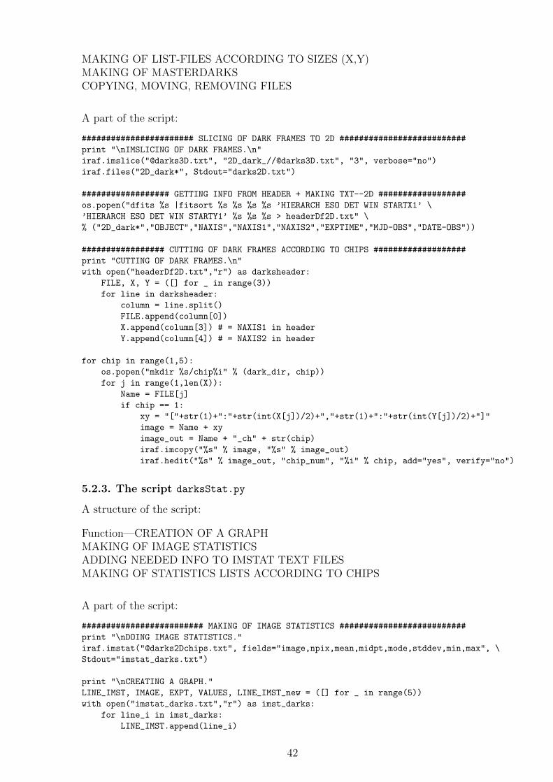
Figure 31: Dependency mean flux on index—dark frames. Size of images:(2048×1130) pix, integration times: left—1.8432 s, bottom right—2.0 s. Each colourof a point in the graphs indicates one of the four chips of the detector.

With longer integration time (lower two images) mean flux should be greater thanwith shorter time but it is not so here. This is because the lower images have got largersize and thereby the mean pixel value is divided by greater number (2,314,240 comparedto 471,040 of upper two images). In terms of images of the same size, the mean flux raiseswith longer integration time as expected.

5.2.2. The script darks.py


OPTION OF DARK FRAMES STATISTICSMAKING OF DARKS LIST FILE (INFO FROM HEADER)SLICING DARK FRAMES TO 2DGETTING INFO FROM HEADER + MAKING OF TXT—2DCUTTING OF DARK FRAMES ACCORDING TO CHIPSGETTING INFO FROM HEADER + MAKING TXT—2D—PARTICULAR CHIPSLAUNCHING DARK STATISTICS SCRIPT IF REQUIRED

41

MAKING OF LIST-FILES ACCORDING TO SIZES (X,Y)MAKING OF MASTERDARKSCOPYING, MOVING, REMOVING FILES


####################### SLICING OF DARK FRAMES TO 2D ##########################

print "\nIMSLICING OF DARK FRAMES.\n"

iraf.imslice("@darks3D.txt", "2D_dark_//@darks3D.txt", "3", verbose="no")

iraf.files("2D_dark*", Stdout="darks2D.txt")

################## GETTING INFO FROM HEADER + MAKING TXT--2D ##################

os.popen("dfits %s |fitsort %s %s %s %s ’HIERARCH ESO DET WIN STARTX1’ \

’HIERARCH ESO DET WIN STARTY1’ %s %s %s > headerDf2D.txt" \

% ("2D_dark*","OBJECT","NAXIS","NAXIS1","NAXIS2","EXPTIME","MJD-OBS","DATE-OBS"))

################# CUTTING OF DARK FRAMES ACCORDING TO CHIPS ###################

print "CUTTING OF DARK FRAMES.\n"

with open("headerDf2D.txt","r") as darksheader:

FILE, X, Y = ([] for _ in range(3))

for line in darksheader:

column = line.split()

FILE.append(column[0])

X.append(column[3]) # = NAXIS1 in header

Y.append(column[4]) # = NAXIS2 in header

for chip in range(1,5):

os.popen("mkdir %s/chip%i" % (dark_dir, chip))

for j in range(1,len(X)):

Name = FILE[j]

if chip == 1:

xy = "["+str(1)+":"+str(int(X[j])/2)+","+str(1)+":"+str(int(Y[j])/2)+"]"

image = Name + xy

image_out = Name + "_ch" + str(chip)

iraf.imcopy("%s" % image, "%s" % image_out)

iraf.hedit("%s" % image_out, "chip_num", "%i" % chip, add="yes", verify="no")

5.2.3. The script darksStat.py


Function—CREATION OF A GRAPHMAKING OF IMAGE STATISTICSADDING NEEDED INFO TO IMSTAT TEXT FILESMAKING OF STATISTICS LISTS ACCORDING TO CHIPS


######################### MAKING OF IMAGE STATISTICS ##########################

print "\nDOING IMAGE STATISTICS."

iraf.imstat("@darks2Dchips.txt", fields="image,npix,mean,midpt,mode,stddev,min,max", \

Stdout="imstat_darks.txt")

print "\nCREATING A GRAPH."

LINE_IMST, IMAGE, EXPT, VALUES, LINE_IMST_new = ([] for _ in range(5))

with open("imstat_darks.txt","r") as imst_darks:

for line_i in imst_darks:

LINE_IMST.append(line_i)

42

col_i = line_i.split()

IMAGE.append(col_i[0])

with open("headerDf2Dchips.txt","r") as head_darks:

for line_h in head_darks:

col_h = line_h.split()

EXPT.append(col_h[8])

VALUES.append((col_h[0],col_h[8], col_h[1]))

EXPTset = set(EXPT[1:])

################### ADDING NEEDED INFO TO IMSTAT TEXT FILES ###################

with open("imstat_darks.txt","w") as imst_darks_w:

row1 = "\t\t\t\t\t%s\t%s\t\t%s" % (LINE_IMST[0][:-1], "EXPTIME", "CHIP_NUM\n")

imst_darks_w.write(row1)

for i in range(len(IMAGE)):

for j in range(len(VALUES)):

if IMAGE[i] == VALUES[j][0]:

row = "%s\t%s\t%s\n" % (LINE_IMST[i][:-1], VALUES[i][1], VALUES[i][2])

LINE_IMST_new.append(row)

imst_darks_w.write(row)

5.3. Flat-field frames

As sensitivity of pixels of a detector is not the same, we remove a sign of this propertyby using flat-field frames. A flat field frame records the response of a detector, so it isactually a map of pixel sensitivity. After we divide an image by a master flat-field frame,the image is corrected about this sign.

Unlike dark frames, flat fields are not taken in Fast Photometry Mode so a flat field isalways 4×[(2048×2048) pix]. Therefore for data reduction it is necessary to cut flat fields(or a master flat field) according to size of science and dark frames.

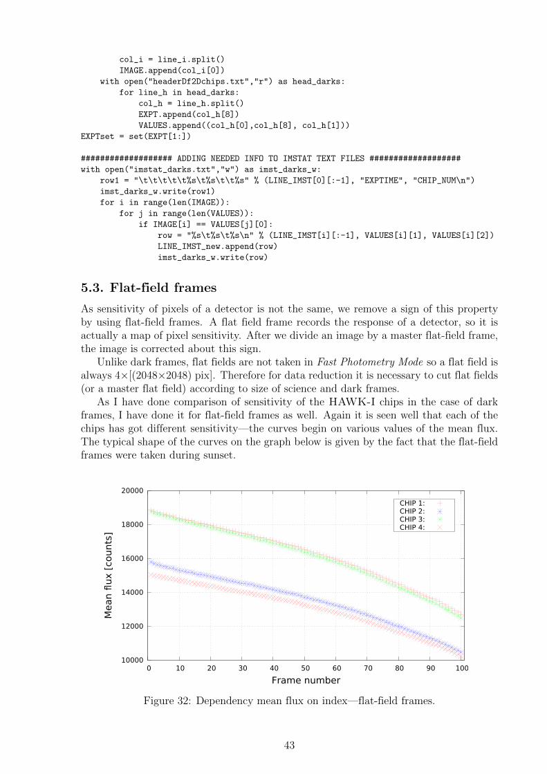
As I have done comparison of sensitivity of the HAWK-I chips in the case of darkframes, I have done it for flat-field frames as well. Again it is seen well that each of thechips has got different sensitivity—the curves begin on various values of the mean flux.The typical shape of the curves on the graph below is given by the fact that the flat-fieldframes were taken during sunset.

10000

12000

14000

16000

18000

20000

0 10 20 30 40 50 60 70 80 90 100

Mean

ux [

counts

]

Frame number


Figure 32: Dependency mean flux on index—flat-field frames.

43

5.3.1. Scripts flats.py and flatsD.py

A structure of the script (the same for both scripts):

OPTION OF FLAT FIELD STATISTICSMAKING OF FLATS LIST FILE (INFO FROM HEADER)LAUNCHING FLAT STATISTICS SCRIPT IF REQUIREDMAKING OF MASTERFLATSEXCHANGING NAMES OF TWO FILES (CHIPS)ADDING NUMBERS OF CHIPS TO MASTERFLATS HEADERSCOPYING, MOVING, REMOVING FILES


########################### MAKING OF MASTERFLATS #############################

print "MAKING OF MASTERFLATS."


list_chip = "@flats2D.txt[" + str(chip) + "]"

image = "mflat_ch"

iraf.imcombine("%s" % list_chip, "%s %i" % (image, chip), combine="median")

# making of master flats

################### EXCHANGING NAMES OF TWO FILES (CHIPS) #####################

iraf.imcopy("mflat_ch3", "mflat_ch3copy")

iraf.imdelete("mflat_ch3") ###> these 6 rows

iraf.imcopy("mflat_ch4", "mflat_ch3") # deal with HAWKI speciality:

iraf.imdelete("mflat_ch4") # extension 4 = chip 3 and

iraf.imcopy("mflat_ch3copy", "mflat_ch4") # extension 3 = chip 4 <###

iraf.imdelete("mflat_ch3copy")

############### ADDING NUMBERS OF CHIPS TO MASTERFLATS HEADERS ################


mflat = "mflat_ch" + str(chip)

iraf.hedit("%s" % mflat, "chip_num", "%i" % chip, add="yes", verify="no")

5.3.2. The script flatsStat.py


Function—CREATION OF A GRAPHCUTTING OF FLATS ACCORDING TO CHIPS + DOING STATISTICSSTATISTICS RESULTS INTO ONE TEXT FILEWRITING OF STATISTICS RESULTS INTO HEADER TEXT FILEMAKING OF LISTS FOR GRAPH ACCORDING TO CHIPS+EXPTIMES


########### CUTTING OF FLATS ACCORDING TO CHIPS + DOING STATISTICS ############

l = [[1,1],[2,2],[4,3],[3,4]] # because ext. 3 = chip 4 and ext. 4 = chip 3

line_num = 0

with open("flats2D.txt","r") as flats2d:

for line in flats2d:

line_num += 1

for i in range(4):

image = line[:-1] + "[" + str(l[i][0]) + "]"

44

list_ch_out = "Flat_" + line[:-1] + "_ch" + str(l[i][1])

iraf.imcopy("%s" % image, "%s" % list_ch_out)

iraf.hedit("%s" % list_ch_out, "chip_num", "%i" % l[i][1], add="yes",

verify="no")

iraf.imstat("%s" % image, fields="image,npix,mean,midpt,mode,stddev,

min,max", Stdout="%s%i%s%i%s" % ("imstat_flats", line_num,

"_ch", l[i][1], txt))

#################### STATISTICS RESULTS INTO ONE TEXT FILE ####################

line_num, ROWS = 0, []

with open("flats2D.txt","r") as flats2d:

for line in flats2d:

line_num += 1


filename_stat = "imstat_flats" + str(line_num) + "_ch" + str(chip) + txt

with open(filename_stat,"r") as stats:

ROWS0 = []

for line in stats:

ROWS0.append(line)

fromRow2 = ROWS0[1:]

ROWS = ROWS + fromRow2

head = ROWS0[0]

with open("imstat_flats_allch.txt","w") as imst_chips:

imst_chips.write(head)

for row in ROWS:

imst_chips.write(row)

5.4. Images before and after reduction compared

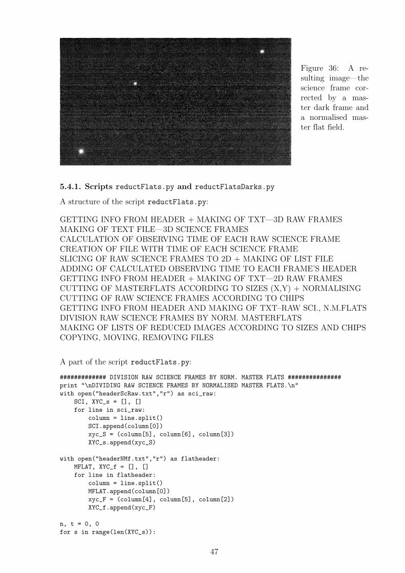
Data reduction consisted of the following steps:

• creating a master dark frame by taking the median of dark frames (with the sameintegration time as science images);• subtracting the created master dark frame from all raw science images [figure 34]

to get dark-corrected science images [figure 35];• creating a master flat field by taking the median of flat fields;• subtracting the master dark from the master flat field to create a dark-corrected

master flat field;• dividing the dark-corrected master flat field by the median of pixel values of this

image to create a normalised master flat field;• dividing all dark-corrected science images by the normalised master flat field to get

resulting images [figure 36].

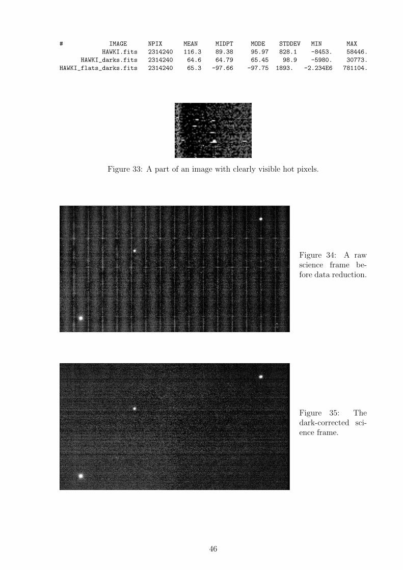
When not using dark frames, raw science frames are corrected only by a normalisedmaster flat field. However, by using them except for dark current elimination we caneliminate also bad pixels and vertical stripes, typical for Fast Photometry Mode. The badpixels are the ones with extremely different values of counts in contrast to the rest of animage (outside stars). Hot pixels (with high values) can be recognised as small white dotsor strips (see figure 33 on the following page).

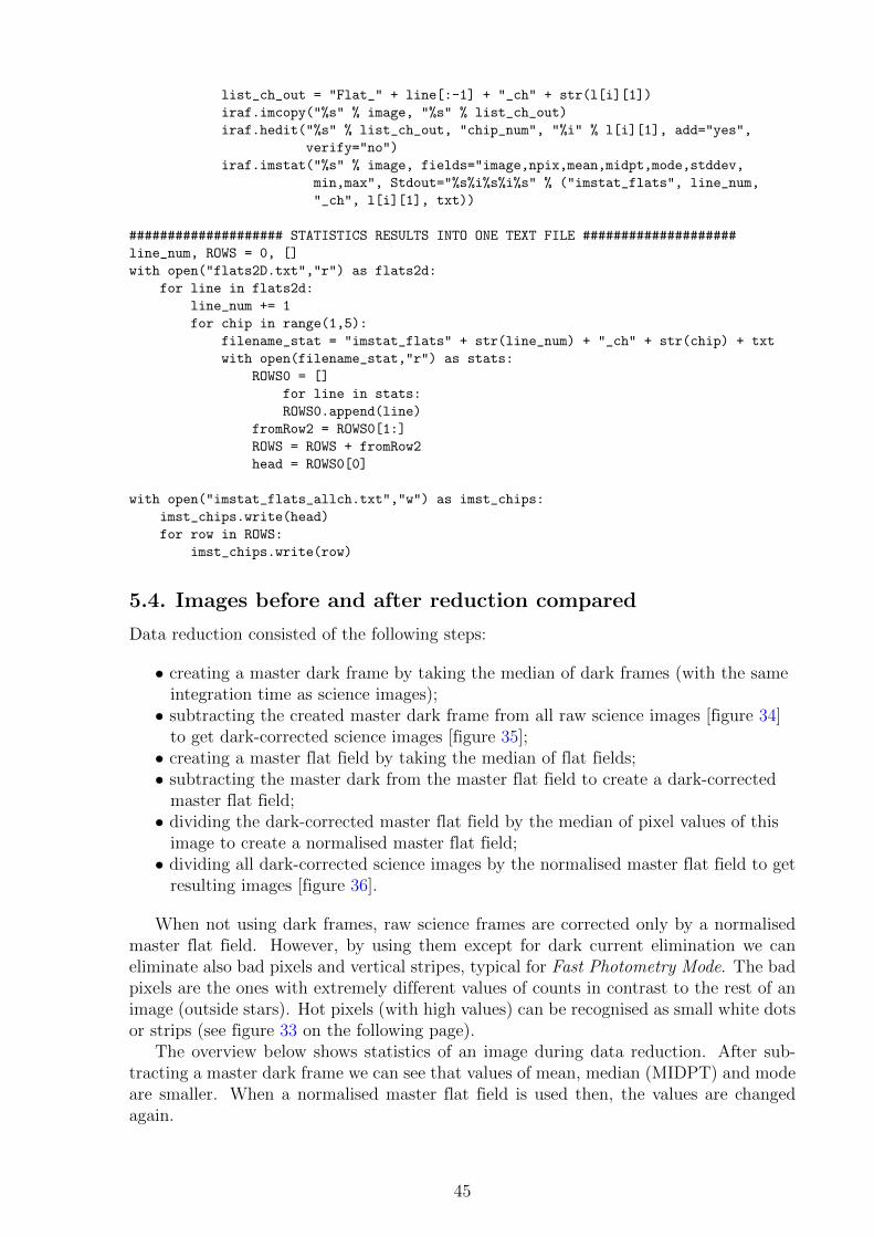
The overview below shows statistics of an image during data reduction. After sub-tracting a master dark frame we can see that values of mean, median (MIDPT) and modeare smaller. When a normalised master flat field is used then, the values are changedagain.

45

# IMAGE NPIX MEAN MIDPT MODE STDDEV MIN MAX

HAWKI.fits 2314240 116.3 89.38 95.97 828.1 -8453. 58446.

HAWKI_darks.fits 2314240 64.6 64.79 65.45 98.9 -5980. 30773.

HAWKI_flats_darks.fits 2314240 65.3 -97.66 -97.75 1893. -2.234E6 781104.

Figure 33: A part of an image with clearly visible hot pixels.

Figure 34: A rawscience frame be-fore data reduction.

Figure 35: Thedark-corrected sci-ence frame.

46

Figure 36: A re-sulting image—thescience frame cor-rected by a mas-ter dark frame anda normalised mas-ter flat field.

5.4.1. Scripts reductFlats.py and reductFlatsDarks.py

A structure of the script reductFlats.py:

GETTING INFO FROM HEADER + MAKING OF TXT—3D RAW FRAMESMAKING OF TEXT FILE—3D SCIENCE FRAMESCALCULATION OF OBSERVING TIME OF EACH RAW SCIENCE FRAMECREATION OF FILE WITH TIME OF EACH SCIENCE FRAMESLICING OF RAW SCIENCE FRAMES TO 2D + MAKING OF LIST FILEADDING OF CALCULATED OBSERVING TIME TO EACH FRAME’S HEADERGETTING INFO FROM HEADER + MAKING OF TXT—2D RAW FRAMESCUTTING OF MASTERFLATS ACCORDING TO SIZES (X,Y) + NORMALISINGCUTTING OF RAW SCIENCE FRAMES ACCORDING TO CHIPSGETTING INFO FROM HEADER AND MAKING OF TXT–RAW SCI., N.M.FLATSDIVISION RAW SCIENCE FRAMES BY NORM. MASTERFLATSMAKING OF LISTS OF REDUCED IMAGES ACCORDING TO SIZES AND CHIPSCOPYING, MOVING, REMOVING FILES

A part of the script reductFlats.py:

############# DIVISION RAW SCIENCE FRAMES BY NORM. MASTER FLATS ###############

print "\nDIVIDING RAW SCIENCE FRAMES BY NORMALISED MASTER FLATS.\n"

with open("headerScRaw.txt","r") as sci_raw:

SCI, XYC_s = [], []

for line in sci_raw:


SCI.append(column[0])

xyc_S = (column[5], column[6], column[3])

XYC_s.append(xyc_S)

with open("headerNMf.txt","r") as flatheader:

MFLAT, XYC_f = [], []

for line in flatheader:


MFLAT.append(column[0])

xyc_F = (column[4], column[5], column[2])

XYC_f.append(xyc_F)

n, t = 0, 0

for s in range(len(XYC_s)):

47

for f in range(len(XYC_f)):

if XYC_s[s] == XYC_f[f]:

sci, mflat = SCI[s], MFLAT[f]

iraf.imarith("%s" % sci, "/", "%s" % mflat, "%s %s" % ("nmf_", sci))

n += 1

if n == 1000:

t += 1

print "Now", n*t, "images done."

n = 0

####### MAKING OF LISTS OF REDUCED IMAGES ACCORDING TO SIZES AND CHIPS ########

print "\nMAKING OF INPUT TEXT FILES FOR PHOTOMETRY."

os.popen("dfits nmf_* |fitsort %s %s > header_file_mjdc.txt" % ("MJD-CALC","EXPTIME"))

os.popen("cp %s %s" % ("header_file_mjdc.txt", "cp_header_file_mjdc.txt"))

os.popen("dfits nmf_* |fitsort %s %s %s %s ’HIERARCH ESO DET WIN STARTX1’

’HIERARCH ESO DET WIN STARTY1’ %s %s %s %s %s ’HIERARCH ESO TEL AMBI FWHM START’

’HIERARCH ESO TEL AIRM START’ %s > header_for_phot.txt" % ("ORIGFILE","NAXIS","NAXIS1",

"NAXIS2","CHIP_NUM","EXPTIME","MJD-CALC","MJD-OBS","DATE-OBS","OBJECT"))

os.popen("cp %s %s" % ("header_for_phot.txt", "cp_header_for_phot.txt"))

with open("header_for_phot.txt","r") as nmf:

FILE0, XYstXstY0, XYstXstYC0 = [], [], []

for line in nmf:


FILE0.append(column[0])

xySTxSTyc = (column[3],column[4],column[5],column[6],column[7])

XYstXstYC0.append(xySTxSTyc)

A structure of the script reductFlatsDarks.py:

GETTING INFO FROM HEADER + MAKING OF TXT—3D RAW FRAMESMAKING OF TEXT FILE—3D SCIENCE FRAMESCALCULATION OF OBSERVING TIME OF EACH RAW SCIENCE FRAMESLICING OF IMAGES TO 2D + MAKING OF LIST FILEADDING CALCULATED OBSERVING TIME TO EACH FRAME’S HEADERGETTING INFO FROM HEADER + MAKING OF TXT—2D RAW SCIENCE FRAMESCUTTING OF MASTERFLATS ACCORDING TO SIZES (X,Y)SUBTRACTION MASTERDARKS FROM MASTERFLATS + NORMALISINGCUTTING OF RAW SCIENCE FRAMES ACCORDING TO CHIPSGETTING INFO FROM HEADER AND MAKING OF TXT—SCI, N.MDARKSUBTRACTION MASTERDARKS FROM SCIENCE RAW FRAMESGETTING INFO FROM HEADER AND MAKING OF TXT—SCI, N.M.FLATD.DIVISION DARK-SUBTR. SCI. FRAMES BY NORM. M.FLATS SUBTR. BY DARKSMAKING OF LISTS OF REDUCED IMAGES ACCORDING TO SIZES AND CHIPSCOPYING, MOVING, REMOVING FILES

A part of the script reductFlatsDarks.py:

########### SUBTRACTION MASTERDARKS FROM MASTERFLATS + NORMALISING ############

print "\nSUBTRACTING MASTERDARKS FROM MASTERFLATS, NORMALISING.\n"

os.popen("dfits m*_*_*_* |fitsort %s %s %s %s %s %s %s > headerMdMf.txt" %

("OBJECT","CHIP_NUM","NAXIS","NAXIS1","NAXIS2","EXPTIME","DATE-OBS"))

with open("headerMdMf.txt","r") as mdarks_mflats:

48

MDARKS, MFLATS = [], []

for line in mdarks_mflats:


if column[1] == "DARK":

MDARKS.append(column[0])

elif column[1] == "FLAT":

MFLATS.append(column[0])

for mflat in MFLATS:

for mdark in MDARKS:

if mflat[6:] == mdark[6:]:

iraf.imarith("%s" % mflat, "-", "%s" % mdark, "%s %s" %

("mflatdark_", mflat[6:]))

iraf.imstat("%s %s" % ("mflatdark_", mflat[6:]),fields="image,npix,

mean,midpt,mode,stddev,min,max", Stdout="%s%s" % ("imst_mfd", txt))

iraf.tbdump("%s %s" % ("imst_mfd", txt), "4", "yes", Stdout="%s%s" %

("MIDPT", txt))

iraf.imarith("%s %s" % ("mflatdark_", mflat[6:]), "/", "%s %s" %

("@MIDPT", txt), "%s %s" % ("n_mflatdark_", mflat[6:])) # norm. m. fl.

############# CUTTING OF RAW SCIENCE FRAMES ACCORDING TO CHIPS ################

print "\nCUTTING OF RAW SCIENCE FRAMES.\n"

with open("headerSc2D.txt","r") as sci_header:

SCI_IM, X, Y, STx, STy = ([] for _ in range(5))

for line in sci_header:


SCI_IM.append(column[0])

STx.append(column[1]) # start X in header

STy.append(column[2]) # start Y in header

X.append(column[3]) # = NAXIS1 in header

Y.append(column[4]) # = NAXIS2 in header

5.5. Bad pixel mask

Chips of detectors have usually got a small amount of bad pixels. If necessary, these canbe removed from data by creating a bad pixel mask. Bad pixel masks show those pixelswhich do not respond linearly. The mask can be created by taking appropriate flat fieldobservations.

It is generated by taking flat field exposures at high and low intensity levels, andidentifying those pixels where the ratio of the normalised flux is more than 15%. For badpixel mask generating IRAF commands imcombine, imarith and ccdmask of IRAF areused (E12). Command fixpix is then used for an application of the generated bad pixelmask on science images. The mask itself is a special type of an image with non-zero valuesfor bad pixels and zero values for good pixels.

Unfortunately, there was no considerable effect after using a bad pixel mask on pro-cessed images. An error could have occured due to the wrong selection of master flats oran inner problem in software. Since the mask had not improved quality of tested images,it was not finally used for data reduction.

49

Figure 37: Bad pixel mask of the chip 3 of HAWK-I.

50

6. Data processing

After basic photometric data reduction is done, we can now start the next step of dataprocessing our data set. The first, and the most important step, is to do photometry, itmeans to measure precisely brightness of stars of our interest. From results of the photo-metry we then create a light curve—dependency of the brightness of a star on time. Themost important step is to analyse the resulting data to obtain physical characterisationof the planetary atmosphere.

The beginning of this chapter describe aperture photometry and how apertures werechosen. The next subsection shows the obtained light curve and the following determinesprecision of photometric measurements. A fitting process of the light curve is describedin the last subsection. As in the previous chapter, structures and parts of Python scriptsappointed for the data processing are always appended.

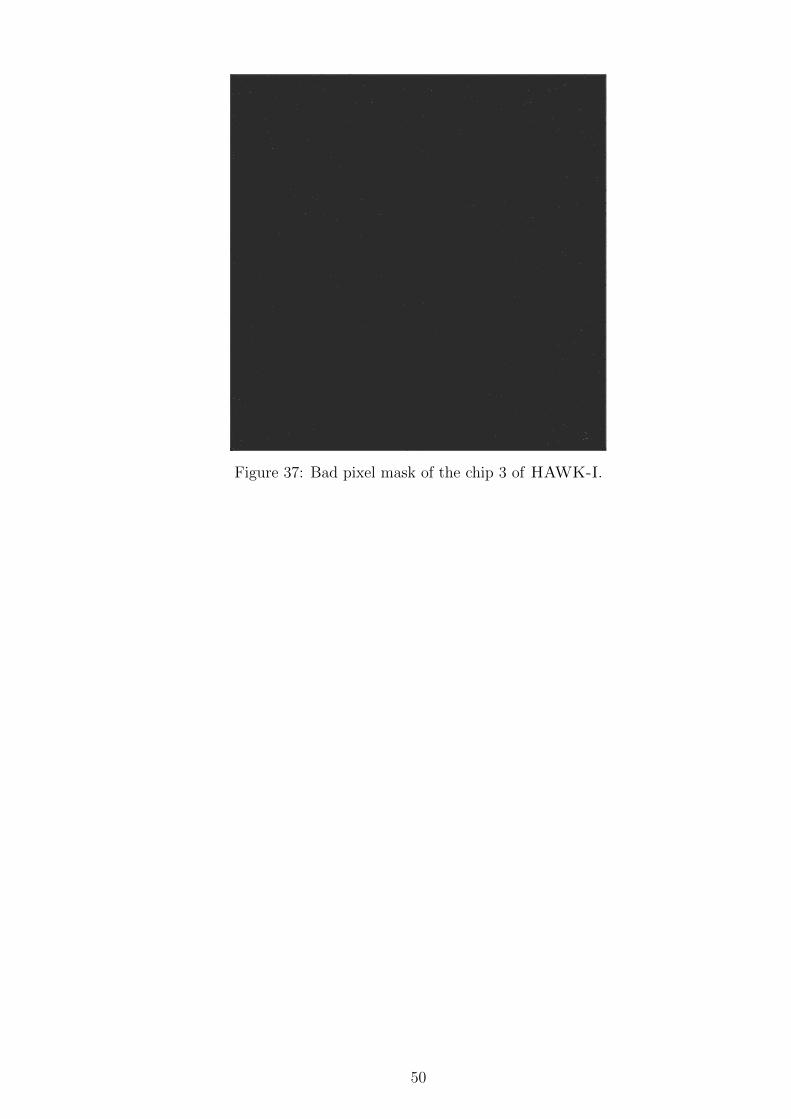
6.1. Aperture photometry

To sum light from a star we use a technique called aperture photometry. To get all the lightfrom the star, we have to determine an aperture radius which should be larger than theapparent size of the star. But a measured value of brightness also includes a contributionof the sky. To subtract it, we have to choose an annulus within sky background with nostar contribution. The size of the annulus is given by inner annulus and outer annulusparameters [figure 38].

Figure 38: The aperture radius capturing light from the star and the annulus to estimatesky background contribution. Taken from Berry and Burnell (2005).

I have done photometry by using phot command in IRAF. An input for the commandis a text file containing list of images required to do the photometry and a text file withcoordinates of measured stars on given images. We usually need to know fluxes for moreaperture radii because we do not know which is the best one and because we measureevery star separately. Therefore it is convenient to write all required aperture radii toanother text file. For an estimate of the aperture radii it is good to look at a few imagesto see what pixel area they occupy.

The phot command contains various settings and apart from the mentioned text files itis necessary to type sizes of annuli to set width of the sky annulus and its distance from thestar. An output of this photometry command is a text file for every single image namedaccording to the image with mag.# suffix where we can find all input parameters andespecially photometry results such as flux, magnitude, x -centre and y-centre positions,etc.

A selection of an optimal aperture is described in following subsection 6.2.

51

6.1.1. The script photometry.py


LOADING NEEDED INFO TO DIFFER SETSFunction—CREATION OF ‘coords.txt’ WITH STARS’ COORDINATESFunction—CREATION OF ‘aperts.txt’ WITH APERTURES TO USENUMBERS OF HAWK-I CHIPS TO USE IN PHOTOMETRYSETTING INPUT TEXT FILES FOR PHOTOMETRYDOING PHOTOMETRYEXTRACTING INFORMATION FROM mag FILESWRITING OF PHOT RESULTS AND OTHER INFO INTO TEXT FILESMAKING OF TEXT FILES WITH THE SAME STARCOPYING, MOVING, REMOVING FILES


##$##$##$## Function-CREATION OF aperts.txt WITH APERTURES TO USE ##$##$##$##$

def aperts_file(imInfo):

with open("aperts_"+imInfo+txt,"w") as apertures:

apert = raw_input("Type apertures which you want to use, separated by comma.\n")

apertures.write(apert)

################ NUMBERS OF HAWK-I CHIPS TO USE IN PHOTOMETRY #################

CHIPS0, CHIPS = [], []

chips = raw_input("\nWhat chips do you want to use for photometry (type numbers separated

by comma)? ")

CHIPS0.append(chips)

for line in CHIPS0:

for chip in line.split(","):

CHIPS.append(chip)

################## SETTING INPUT TEXT FILES FOR PHOTOMETRY ####################

ALLINFO, ALLSTARS = [], []

for chip in CHIPS:

for el in XYXYset:

i, star, STARS0, INFO = 1, str, [], []

x, y, STx, STy = str(el[0]), str(el[1]), str(el[2]), str(el[3])

imInfo = x + "_" + y + "_" + STx + "_" + STy + "_" + chip

INFO.append(imInfo)

print "\n" + ">" + 15 * "-" + ">"

while star != "f": # even if there’s no star on an image, ’coords’ and

’aperts’ files must be created (empty)!

star = raw_input("Write a name of " + imInfo + " set of the " + str(i)

+ ". star (when finished, type ’f’): ")

i += 1

STARS0.append(star)

ALLSTARS.append(star)

STARS = STARS0[:-1]

INFO.append(STARS)

ALLINFO.append(INFO)

52

6.2. Apertures

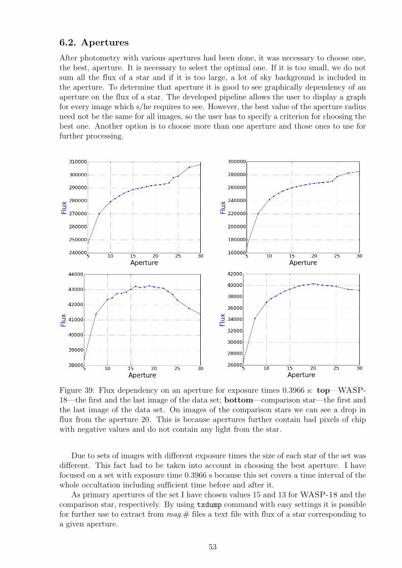
After photometry with various apertures had been done, it was necessary to choose one,the best, aperture. It is necessary to select the optimal one. If it is too small, we do notsum all the flux of a star and if it is too large, a lot of sky background is included inthe aperture. To determine that aperture it is good to see graphically dependency of anaperture on the flux of a star. The developed pipeline allows the user to display a graphfor every image which s/he requires to see. However, the best value of the aperture radiusneed not be the same for all images, so the user has to specify a criterion for choosing thebest one. Another option is to choose more than one aperture and those ones to use forfurther processing.

Figure 39: Flux dependency on an aperture for exposure times 0.3966 s: top—WASP-18—the first and the last image of the data set; bottom—comparison star—the first andthe last image of the data set. On images of the comparison stars we can see a drop influx from the aperture 20. This is because apertures further contain bad pixels of chipwith negative values and do not contain any light from the star.

Due to sets of images with different exposure times the size of each star of the set wasdifferent. This fact had to be taken into account in choosing the best aperture. I havefocused on a set with exposure time 0.3966 s because this set covers a time interval of thewhole occultation including sufficient time before and after it.

As primary apertures of the set I have chosen values 15 and 13 for WASP-18 and thecomparison star, respectively. By using txdump command with easy settings it is possiblefor further use to extract from mag.# files a text file with flux of a star corresponding toa given aperture.

53

6.2.1. The script aperts.py


Function—CREATION OF A GRAPH APERTS VS. FLUXESCHECK FOR POSSIBLE OLD FILESFunction—CHOICE OF THE BEST APERTURECHOICE OF STARS FOR A LIGHT CURVE AND BEST APERTURE GRAPHCHOICE OF STARS’ APERTURES FOR THE LIGHT CURVECOPYING, MOVING, REMOVING FILES


######### CHOICE OF STARS FOR A LIGHT CURVE AND BEST APERTURE GRAPH ###########

LC_STARS = []

for i in range(1,3):

lc_star = raw_input("Write a name of the " + str(i) + ". star for a light curve

(1st / 2nd): ")

LC_STARS.append(lc_star)

ask_ap = raw_input("\nDo you want to show a graph of apertures vs. fluxes (if not,

type ’n’)? ")

if ask_ap != "n":

best_apert(LC_STARS)

################### CHOICE OF STARS’ APERTURES FOR THE LIGHT CURVE #####################

check_files()

LINES, ALL, star_count = [], [], 0

for star in LC_STARS:

star_count += 1

ap_filename = phot_out + star + txt

FLUXES_LIST, APS_LIST = [], []

with open(ap_filename,"r") as lc_ap:

for line in lc_ap:

row = line.split()

num_aps = (len(row) - 6) / 2

ALLAPS, APS, APS0 = [], [], row[-num_aps:]

for a in APS0:

APS.append(float(a))

num_fluxes_end = ((len(row) - 6) / 2) + 6

FLUXES, FLUXES0 = [], row[6:num_fluxes_end]

6.3. Light curve

In this section, after data reduction, photometry and the best aperture selection, thepipeline creates a light curve, the most important result. To get the final light curve,a few steps preceded. They will be described below.

As observation time of images written in their header is in Modified Julian Date(MJD), to convert MJD to Barycentric Julian Date of Barycentric Dynamical Time(BJD TDB) I had recalculated it to Julian Date (JD) and then I used an online utility(E18) which converted JD of observations to BJD.

54

A creation of light curves consisted of a few steps:

• image by image to divide flux of a target star by flux of a comparison star (1 or 2)to make a ratio of fluxes;• from a set of calculated ratios of all images exclude those belonging to images ob-

tained during an eclipse;• take the median of fluxes ratios of remaining images of the set;• to divide fluxes ratios of all the images by the median to calculate normalised ratio

of fluxes;• to plot a light curve—a graph showing dependency of the normalised ratio of fluxes

on time.

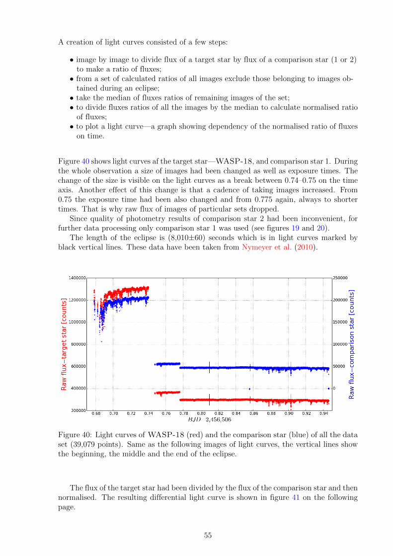
Figure 40 shows light curves af the target star—WASP-18, and comparison star 1. Duringthe whole observation a size of images had been changed as well as exposure times. Thechange of the size is visible on the light curves as a break between 0.74–0.75 on the timeaxis. Another effect of this change is that a cadence of taking images increased. From0.75 the exposure time had been also changed and from 0.775 again, always to shortertimes. That is why raw flux of images of particular sets dropped.

Since quality of photometry results of comparison star 2 had been inconvenient, forfurther data processing only comparison star 1 was used (see figures 19 and 20).

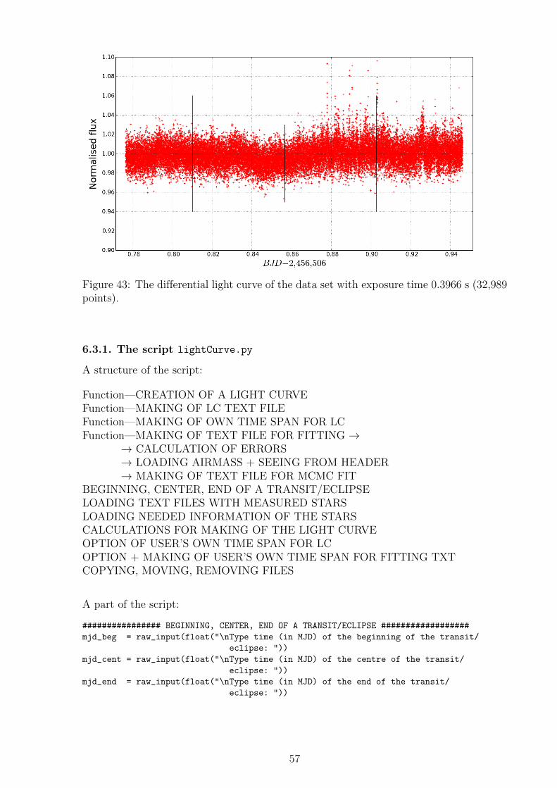
The length of the eclipse is (8,010±60) seconds which is in light curves marked byblack vertical lines. These data have been taken from Nymeyer et al. (2010).

Figure 40: Light curves of WASP-18 (red) and the comparison star (blue) of all the dataset (39,079 points). Same as the following images of light curves, the vertical lines showthe beginning, the middle and the end of the eclipse.

The flux of the target star had been divided by the flux of the comparison star and thennormalised. The resulting differential light curve is shown in figure 41 on the followingpage.

55

Figure 41: The differential light curve of all the data set (39,079 points)—WASP-18 /comparison star. Density of points increased after size of images had been reduced. Thegap between BJD 0.74 and 0.75 is due to the change of the size of the images (andexposure time).

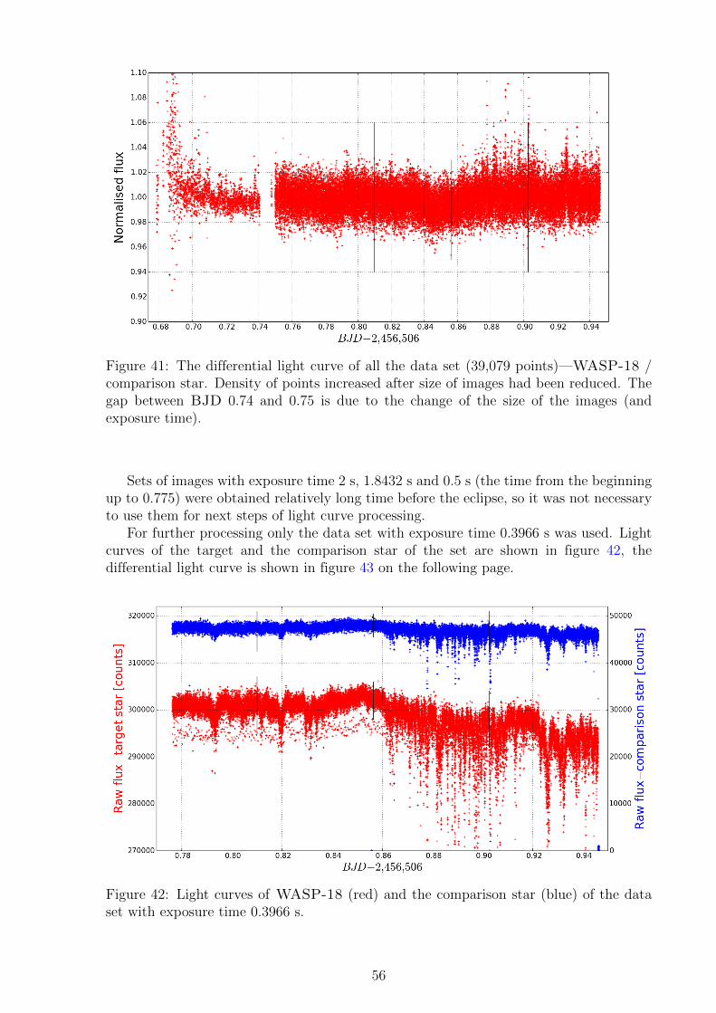
Sets of images with exposure time 2 s, 1.8432 s and 0.5 s (the time from the beginningup to 0.775) were obtained relatively long time before the eclipse, so it was not necessaryto use them for next steps of light curve processing.

For further processing only the data set with exposure time 0.3966 s was used. Lightcurves of the target and the comparison star of the set are shown in figure 42, thedifferential light curve is shown in figure 43 on the following page.

Figure 42: Light curves of WASP-18 (red) and the comparison star (blue) of the dataset with exposure time 0.3966 s.

56

Figure 43: The differential light curve of the data set with exposure time 0.3966 s (32,989points).

6.3.1. The script lightCurve.py


Function—CREATION OF A LIGHT CURVEFunction—MAKING OF LC TEXT FILEFunction—MAKING OF OWN TIME SPAN FOR LCFunction—MAKING OF TEXT FILE FOR FITTING →

→ CALCULATION OF ERRORS→ LOADING AIRMASS + SEEING FROM HEADER→ MAKING OF TEXT FILE FOR MCMC FIT

BEGINNING, CENTER, END OF A TRANSIT/ECLIPSELOADING TEXT FILES WITH MEASURED STARSLOADING NEEDED INFORMATION OF THE STARSCALCULATIONS FOR MAKING OF THE LIGHT CURVEOPTION OF USER’S OWN TIME SPAN FOR LCOPTION + MAKING OF USER’S OWN TIME SPAN FOR FITTING TXTCOPYING, MOVING, REMOVING FILES


################ BEGINNING, CENTER, END OF A TRANSIT/ECLIPSE ##################

mjd_beg = raw_input(float("\nType time (in MJD) of the beginning of the transit/

eclipse: "))

mjd_cent = raw_input(float("\nType time (in MJD) of the centre of the transit/

eclipse: "))

mjd_end = raw_input(float("\nType time (in MJD) of the end of the transit/

eclipse: "))

57

################### LOADING TEXT FILES WITH MEASURED STARS ####################

os.popen("ls %s > %s%s" % (main_dir, "files", txt)) # writes names of files and

folders to a text file

with open("files"+txt,"r") as lc_files:

for line in lc_files:

if line[:7] == "1st_lc_":

File1 = line[:-1]

elif line[:7] == "2nd_lc_":

File2 = line[:-1]

os.popen("rm %s%s" % ("files", txt))

################## LOADING NEEDED INFORMATION OF THE STARS ####################

LINES1, LINES2, EXPT1, EXPT2, MJD1, MJD2, FLUX1, FLUX2, FLUX_ratio,\

Xcent1, Xcent2, Ycent1, Ycent2 = ([] for _ in range(13))

with open(File1,"r") as lc1: # target star

for line1 in lc1:

star1 = File1[7:-4]

LINES1.append(line1)

col1 = line1.split()

EXPT1.append(col1[0])

MJD1.append(col1[1])

FLUX1.append(float(col1[2]))

Xcent1.append(col1[3])

Ycent1.append(col1[4])

with open(File2,"r") as lc2: # comparison star

for line2 in lc2:

star2 = File2[7:-4]

LINES2.append(line2)

col2 = line2.split()

EXPT2.append(col2[0])

MJD2.append(col2[1])

FLUX2.append(float(col2[2]))

Xcent2.append(col2[3])

Ycent2.append(col2[4])

6.4. Standard deviation

To investigate quality and stability of a light curve, a statistical measure called standarddeviation is used. To calculate the standard deviation of a measurement, we use thefollowing formula:

σ =

√√√√ 1

N

N∑i=1

(xi − x)2.

Here xi are observed values, x is the mean value of all observations and N is thenumber of values.

I have calculated standard deviations for a few data sets. All sets are of exposure time0.3966 s. The first one is the set with all points (used for the light curve in figure 43). Thesecond set (marked as “binned-s”) contains points limited by known seeing (see figure 45and details in subsection 6.5.). The third set results from the second set but data arebinned by 30 seconds. The last set is the same but binned by 2 min (see figure 46). Forall the data sets I have have calculated the deviations for a few time intervals to see howit changes with time. The points implied in the calculations must not cover any part ofthe occultation so that results would not be affected by a change of flux caused by theoccultation. Table 5 compares the calculated standard deviations for the mentioned datasets.

58

Time intervalBinning 30 s 1 min 2 min 5 min 10 min

unbinned 0.0092 0.0095 0.0094 0.0094 0.0094unbinned-s 0.0048 0.0062 0.0059 0.0087 0.0101

30 s 0.0038 0.0044 0.0048 0.0051 0.0061120 s — — 0.0023 0.0019 0.0034

Time intervalBinning 15 min 20 min 30 min 40 min all data

unbinned 0.0096 0.0096 0.0100 0.0101 0.0113unbinned-s 0.0105 0.0099 0.0104 0.0112 0.0135

30 s 0.0064 0.0064 0.0072 0.0077 0.0084120 s 0.0037 0.0037 0.0043 0.0046 0.0051

Table 5: Calculated standard deviations. Unbinned : all points; unbinned-s : points limitedby known seeing; 30 s : the same points as the previous, binned by 30 s; 120 s : the same,binned by 2 min.

As the analysis shows, the precision is in order of millimagnitudes and it is better ifbinning of data is used. The best stability of the light curve is reached on bin 2 minutesover an interval of 5 minutes with its value of 0.0019. In addition, the light curve isslightly corrected by a polynomial during fitting. We can also notice that with longertime intervals the precision becomes worse. Quality of the data had worsened and thevariance increased. It is probably caused by repeated changes of seeing which becameboldly worse during the occultation (see figure 24).

Figure 44: Standard deviation for different time intervals calculated for the unbinneddata (blue), unbinned data with the seeing limitation (green), the same data binned by30 s (red) and by 2 min (black).

59

A larger bin width means better signal-to-noise ratio, however, it also contributes toa larger value of red noise. This makes precision and stability of a light curve worse.The impact of the red noise of our data is shown on graph 49 in section 6.5. If there isonly white noise, the graph would be a line but the red noise deviates the curve from thestraight line.

6.4.1. The script std.py


LOADING NEEDED LC FILE + INFO FROM THATSETTING OF INTERVALS + STARTING POINT FOR CALCULATIONMAKING OF LISTS FOR CHOSEN INTERVALSCALCULATION OF A STANDARD DEVIATIONMAKING OF TEXT FILE WITH RESULTSPRINTOUT OF A TABLE WITH RESULTSCOPYING, MOVING, REMOVING FILES


############ SETTING OF INTERVALS + STARTING POINT FOR CALCULATION #############

TM, MINS, SIGmed, SIGmean = ([] for _ in range(4))

time = raw_input("Type in minutes (separated by comma) intervals to determine

standard deviation: ")

TM.append(time)

start_ask = raw_input("\nDo you want to start from the first point of the data

set or type your own time (if own, type ’o’): ")

if start_ask == "o":

start_point = float(raw_input("\nType your MJD time: "))

start = start_point

else:

start = min(Pair)

#################### MAKING OF LISTS FOR CHOSEN INTERVALS #####################

step = 1.0 / 86400 # step per one second

for line in TM:

for minute in (line.split(",")):

MINS.append(minute)

FLUX = []

t = float(minute) * 60 # time in seconds

Range = t * step # range of data for RMS

end = start + Range # ending point in MJD

if end > max(Pair):

print "\nThe last point is on " + str(max(Pair)) + "."

for date in Pair: # 1st item of each pair in dict.

if start <= date <= end:

FLUX.append(Pair[date])

60

6.5. Fitting

For fitting of the resulting data I used Markov Chain Monte Carlo (MCMC) fittingmethod. MCMC methods in Bayesian statistics (called after English statistician) arealgorithms to sample from a probability distribution. It is based on stochastic simulationsand on constructing a chain (called Markov after Russian mathematician) with the desireddistribution. After a number of steps the state of the chain is then used as a sample ofthe desired distribution. The higher the number of steps the better quality of the sample.Since this case involves a planet orbiting a star, the model used for fitting is based onKeplerian orbit about a centre of mass of theirs. The used routine has been kindly providedby Michael Gillon. It is closely described in (Gillon et al., 2009). Before an eclipse if beingmodelled, by using polynomials with low order the light curve is detrended. They can bealso used to remove atmospheric extinction, correct positions of the star on the detectoror eventually seeing.

Since to fit a light curve created of consecutive points of about 0.4 s (the case of all32,989 points) is very demanding for a computer and it is not necessary to fit such detaileddata, some criteria to exclude a lot of points was needed to determine. One of entries ofan input file for MCMC method of fitting is seeing. As previously mentioned, a value ofseeing is known only for the first and the last image of each of cube fits files. This wasa good criterion to choose points for the light curve fitting. I have chosen the first imageof every cube of the data set covering the eclipse. It consisted of 654 points.

Figure 45: The normalised light curve of the data set with exposure time 0.3966 s createdof the first images of each of cubes (654 points).

The input text file for fitting by MCMC code requires 7 columns with respectivelythese entries: time, a normalised ratio of fluxes, an error of the fluxes, a position of thetarget star on x-axis, a position of the target star on y-axis, airmass, seeing.

Before fitting is started, except creating the input file parameters of a system andother settings have to be set (in a file mcmc.dat). This model of MCMC fitting methodallows to fit various physical characteristics but the interest was just to estimate the

61

eclipse depth, which is equal to a ratio of flux of the planet above flux of the star, so thisonly fit option was set to yes.

I launched the fitting procedure with various settings and with different input files(unbinned with 654 points or binned with smaller number of points). The fitting bestconverged when binning of 2 minutes was used. This corresponds to 120 points (figure 46).The setting of the mcmc.dat file was following:

|-----------------------------------------------------------------------|

|MARKOV-CHAINS: |

|-----------------------------------------------------------------------|

|NUMBER_OF_CHAINS: 3 |

|LENGTH_OF_EACH_CHAIN: 100000 |

|BURN-IN_PHASE: 300 |

|STAT_LENGTH: 50 |

|RED_NOISE_TIMESCALES_(MIN): 10 |

|BIN_SIZE_OF_GLOBAL_FOLDED_LC_(MIN): 10 |

|DESIRED_SUCCESS_RATE: 0.25 |

|SERIES_OR_NUMERICAL_SOLUTION_TO_KE(s_or_n)? n |

|PRECISION_OF_KE_NUMERICAL_SOLUTION: 1.E-8 |

|GIBBS_SAMPLER(y_or_n)? y |

|GLOBAL_ADAPTATION_OF_JUMPS(y_or_n)? y |

|MAXADAPT(min=1) 1.E3 |

|GELMAN-RUBIN_TEST?: y |

|COMPUTATION_OF_MARGINAL_LIKELIHOOD(y_or_n)? y |

|TTV_MINIMIZE(y_or_n)? n |

|ALLOW_FOR_DDFs(y_or_n)? n |

|NUMBER_OF_PLANETS: 1 |

|MINIMAL_PERIOD_(DAYS): 0.5 |

|MAXIMAL_PERIOD_(YEAR): 0.006 |

|MINIMAL_PLANET_RADIUS_(R_jup)+SIGMA: 0.001 0.54 |

|MAXIMAL_PLANET_RADIUS_(R_jup)+SIGMA: 5.3 0.54 |

|TRANSIT_DILUTION+ERROR_(%): 0. 0. |

|-----------------------------------------------------------------------|

|DATA: |

|-----------------------------------------------------------------------|

|NUMBER_OF_PHOTOMETRIC_TIME-SERIES: 1 |

| N F A B_o C_o D_o E F G TTV Beta WS |

| 1 120 J+K s y 1 y 1 n 0 n n n n 1.2 n |

| |****************************************|

| | N=number of points |

| | F=filter [S+uvby,J+UBVRIJHK,ugriz+’] |

| | A=eclipse nature(p or s) |

| | B_o=model extinction?[y/n+order’(1-4)] |

| | C_o=model trend?[y/n+order(0-4)] |

| | D_o=model of X[7]?[y/n+order(0-4)] |

| | E=model IRAC/IRS ramp?[y/n] |

| | F=model IRAC phase-pixel?[y/n] |

| | G=model IRAC WS phase-pixel?[y/n] |

| | TTV=fit a TTV for this eclipse?[y/n] |

| | DF=fit delta transit depth?[y/n] |

| | Beta=Error correction factor[>=1] |

| | WS=write baseline PDF?[y/n] |

| |****************************************|

|OCC: DEPTH + ERROR, DILUTION + ERROR + FIT OPTION[y,n,p]: |

| 1 0.001 0.1 0.0 0.0 y |

|NUMBER_OF_RV_TIME-SERIES_+_TREND_OPTION[y_or_n+order] 0 n 0 |

| N JITTER[m/s] POLYORDER |

|NUMBER_OF_TRANSIT_TIMINGS: 0 n |

|NUMBER_OF_OCCULTATION_TIMINGS: 1 n |

|-----------------------------------------------------------------------|

|INITIAL VALUES + ERRORS + FIT OPTIONS[y,n,p] |

|-----------------------------------------------------------------------|

|DF_+_ERROR: 0.00917 0.0002 n |

|IMPACT_PARAMETER_+_ERROR: 0.527 0.052 n |

|ECLIPSE_DURATION_+_ERROR_(day): 0.0927083 0.000694 n |

|T0_+_ERROR_(BJD): 6506.3855 0.2 n |

|PERIOD_+_ERROR_(day): 0.9414523 0.0000004 n |

|EXCENTRICITY_+_ERROR: 0.0091 0.0012 n |

|OMEGA_+_ERROR_(degree): -91. 3. n |

|ERROR_SQRT(E)COSW+SQRT(E)SINW 0. 0. n |

|K_+_ERROR_(ms-1): 0. 0. n |

|BETA_+_ERROR_(degree): 0. 0. n |

62

|ERROR_VSINICOSB+SINB: 0. 0. n |

|-----------------------------------------------------------------------|

|OPTIONS [y/n] !

!-----------------------------------------------------------------------!

|MODEL_ROSSITER_EFFECT? n |

|PRIOR_ON_THE_STELLAR_DENSITY? n |

|FIX_THE_STELLAR_RADIUS_AND_MASS? n |

!PRIOR_ON_VSINI? n |

!PRIOR_ON_LOGG? n |

!USE_TORRES_STELLAR_CALIBRATION? n |

|-----------------------------------------------------------------------|

|LIMB-DARKENING |

|-----------------------------------------------------------------------|

|LIMB-DARKENING_LAW_[qd,nl,no] no |

|INTERPOLATE_LD_COEFFICIENTS_FROM_TABLE?_[y,n] n |

|-----------------------------------------------------------------------|

|SPECTROSCOPIC PARAMETERS |

|-----------------------------------------------------------------------|

|TEFF_+_ERROR_(K): 6400.0 100.0 |

|LOGG_+_ERROR: 4.4 0.15 |

|[FEH]_+_ERROR: 0.00 0.09 |

|VTURB_+_ERROR_(kms-1): 4.8 0.3 |

|VSINI+_ERROR_(kms-1): 11.0 1.5 |

|-----------------------------------------------------------------------|

|STELLAR PARAMETERS (USED ONLY IF PRIOR ON THE DENSITY) |

|-----------------------------------------------------------------------|

|MASS_+_ERROR_(Msun): 1.28 0.09 |

|RADIUS_+_ERROR_(Rsun): 1.29 0.16 |

|-----------------------------------------------------------------------|

Figure 46: The differential light curve of the data set with exposure time 0.3966 s createdfrom the first images of each of cubes. This curve is binned by 2 min (120 points) andwas used for fitting.

The fitting procedure best converged when polynomials to model extinction and todetrend the light curve were of first order. The occultation depth (δocc) was determinedto be 0.0036+0.0023

−0.0021, in other words, when the planet is hidden behind its host star, thetotal flux of the system decreases by about 0.36%. In comparison with other observationspublished in papers (Nymeyer et al. (2010), Iro and Maxted (2013)) the eclipse depth islarger than expected.

63

The fitted light curve and residuals from the best-fitting model are shown in figures47 and 48.

Figure 47: Detrended light curve and the best-fitting model of the occultation of exoplanetWASP-18b. The eclipse depth has been determined to be 0.36 %.

Figure 48: Residuals from the best-fitting model. The standard deviation is 0.0052.

Figure 49 on the following page shows a red noise diagram for the residuals. For variousbin widths fitting models had been made. We can see that for larger bin widths, startingat about 20 minutes, the red noise begins to be dominating over the white noise—thecurve begins to deviate from the line. This results in the fact that the range of applicablebin widths is limited.

64

Figure 49: Red noise diagram for the residuals of fitting models. The points on the linerepresent the standard deviations calculated for a given bin width.

6.6. Discussion of the atmosphere of WASP-18b

Figure 50 shows a model of the atmosphere of WASP-18b (previously shown at sub-section 1.3.1.). The occultation model obtained by the data processed in this thesis wasadded and it is marked by brown. The expected depth for wavelength 2.09 µm (the usedfilter) was according to the model slightly over 0.002 but the fitted depth is 0.0036+0.0023

−0.0021.However, this is the first result. A subject of further study will be thorough check of po-tential instrument effects.

Figure 50: Dayside spectrum of WASP-18b made of observations of Spitzer’s InfraredArray Camera. It is the same as shown in subsection 1.3.1. but this also includes theresults of the fitting process done in this thesis. The brown circle with an error bar is theresult which was determined to be 0.0036 but the expected depth had been about 0.002.Adapted from Nymeyer et al. (2010).

65

The atmosphere of WASP-18b including the heat redistribution was recently studiedand published in (Iro and Maxted, 2013). Since the planet is highly irradiated by itshost star, one of their input parameters had been temperature inversion on the day-side.The inversion is supposed to be caused by molecules of TiO and V O which in such hightemperatures exist in gas phase. The model was calculated for no rotation and for a fastdifferential rotation of the atmosphere. The rotation model resulted in heat redistributionover the whole planet whereas no rotation model showed higher temperature contrastsbetween the day-side and the night-side. In the case of no rotation of the atmosphere, thetemperature of the day-side is higher than in the rotation case. Then the observed flux ofthe day-side is higher and consequently the occultation depth as well. No rotation modelalso matches to the data of the occultation from Nymeyer et al. (2010). Furthermore,when the substellar point (the direction of the star) is exactly facing the Earth, the fluxof the planet increases. Another effect affecting the heat redistribution is latitudinaltransport of the heat. However, this was not included in the calculations of the model.These mentioned effects may be possible reasons why our occultation depth is larger thanexpected.

The results of this thesis are preliminary. Further, more detailed processing, enableus to detrend the light curve better which will enhance precision of our measurements.

66

7. Conclusion

The main aim of this thesis was to develop software able to process photometric datafrom reduction up to creating a light curve and preparing resulting data for fitting. Thedeveloped pipeline is made of a few Python scripts allocated according to their functions.After one script ends, the next one is launched. The pipeline is appointed for Fast Photo-metry Mode where input files/images are 3D cubes. However, after some modificationsit could be used to process images not taken by FPM. Some scripts require co-operationwith a user, especially those concerning photometry. A detailed description of the pipelineis found in Appendix on page 71.

The software was successfully tested on photometric data of an occultation of systemWASP-18, obtained 1.–2. 8. 2013 on ESO Paranal by Very Large Telescope with NIRinstrument HAWK-I. The data set consists of four particular sets differing by sizes andespecially by exposure times. They contain images with the target star (WASP-18b)a two comparison stars. However, since comparison star 2 could not be used for itsinconvenient quality, to create a differential light curve only comparison star 1 could havebeen used. The first three data sets were not been finally used for processing becausethey had been taken long time before the occultation. The original number of images hadbeen 39,079. Due to the mentioned reasons and by using a seeing criterion and binningof 2 min, the number of points for the light curve was reduced to 120. After the datareduction and processing had been done, an output of the software was a text file withexactly given structure required by MCMC method of fitting.

Quality of images was affected (among others) by seeing which became worse in aboutthe second half of the eclipse. This is obvious from results of photometry and from theprecision analysis. In this stage, an occultation of the planet by its host star has beendetected. The detected occultation depth is 0.0036+0.0023

−0.0021 which is larger than expectedwhen compared to models published in cited publications but it is a clear detection.

In further steps, we need to investigate the nature of such a deep eclipse and try toexplain it. Discussion of the photometric precision and more extensive investigation ofred noise analysis will be the subject of further analysis along with modelling of an eclipsewith a method of Gaussian processes (Gibson et al., 2011). In addition, physical processessuch as heat redistribution in the planet surface or potential presence of gasses like TiOand will be taken into account, too. There are various effects on the observed flux of thesystem during an occultation such as rotation of the atmosphere, position of the day-sideof the planet towards an observer, etc. (Iro and Maxted, 2013).

These are first results which will be the subject of further study. After the thoroughstudy is done, the results are intended to be published in a paper.

67

Bibliography

Berry, R., Burnell, J.: The handbook of astronomical image processing. Richmond (USA),Willmann-Bell, Inc., 2005, ISBN 0-943396-82-4. 51

Blazek, M.: Bakalarska prace: CCD fotometrie tranzitujıch extrasolarnıch planet. Brno,Faculty of Science of Masaryk University, 2014.

Boss, A. P., et al.: Working Group on extrasolar planets. Reports on astronomy, proceed-ings IAU symposium No. XXVIA, 183–186. International Astronomical Union, 2007. 13

Bouy, H., et al.: Multi-conjugate adaptive optics images of the Trapezium cluster. Astron-omy & Astrophysics. ESO, 2013. 33

Charbonneau, D., et al.: Detection of planetary transits across a Sun-like star. The As-trophysical Journal, volume 529, L45–L48. The American Astronomical Society, USA,2000. 14, 16

Dragomir, D., et al.: Rayleigh scattering in the atmosphere of the warm exo-NeptuneGJ 3470B. The Astrophysical Journal, volume 814, number 2, 2015. 19

Gibson, N., P., et al.: A Gaussian process framework for modelling instrumental system-atics: application to transmission spectroscopy. Monthly Notices of the Royal Astro-nomical Society, 2011. 67

Gillon, M., et al.: VLT transit and occultation photometry for the bloated planet CoRoT-1b, 1–10. Astronomy & Astrophysics, 2009. 61

Hellier, C.: An orbital period of 0.94 days for the hot-Jupiter planet WASP-18b. Nature,volume 460, 1098–1100. Letters to Nature, 2009. 18

Huygens, C.: Cosmotheoros. Adriaan Moetjens, The Hague, 1698. 12

Iro, N., Maxted, P. F. L.: On the heat redistribution of the hot transiting exoplanet WASP-18b. Icarus, volume 226, issue 2, 1719–1723, 2013. 19, 63, 66, 67

Van de Kamp, P.: Astrometric study of Barnard’s star from plates taken with the 24-inchsproul refractor. The Astronomical Journal, volume 68, number 7, 515–521, USA, Amer-ican astronomical society, 1963. 12

Knutson, H. A.: A map of the day-night contrast of the extrasolar planet HD 189733b.Nature, volume 447, 183–186. Letters to Nature, 2007. 21

Mayor, M., Queloz, D.: A Jupiter-mass companion to a solar-type star. Nature, volume378, issue 6555, 355–359. Geneva observatory, Switzerland, 1995. 12, 16

Nymeyer, S., et al.: Spitzer secondary eclipses of WASP-18b. The Astrophysical Journal,2010. 18, 20, 55, 63, 65

Seager, S.: Exoplanets. Arizona (USA), The University of Arizona Press, 2010,ISBN 978-0-8165-2945-2. 12

68

Seager, S.: Exoplanet Atmospheres (Physical Processes). Princeton–New Jersey (USA),Princeton University Press, 2010, ISBN 978-0-691-14645-4. 19

Seager, S., Deming, D.: Exoplanet atmospheres. Astronomy & Astrophysics, volume 48,631–672. ESO, 2010.

Seager, S., Mallen-Ornelas, G.: On the unique solution of planet and star parametersfrom an extrasolar planet transit light curve. The Astrophysical Journal, 585: 1038–1055. USA, The American astronomical society, 2003. 22

Vidal-Madjar, A., et al.: An extended upper atmosphere around the extrasolar planetHD209458b. Nature, volume 422, 143–146. Letters to Nature, 2003. 19

Winn, J. N.: Transits and occultations. Massachusetts Institute of Technology, 2010. 21, 23

Wolszczan, A., Frail, D. A.: A planetary system around the millisecond pulsarPSR1257+12. Nature, volume 355, 145–147. Letters to Nature, 1992. 12

69

Internet sources

[E0] http://visibleearth.nasa.gov/

[E1] http://www.iau.org/

[E2] http://www.exoplanet.eu/

[E3] http://exoplanets.org/

[E4] https://corot.cnes.fr/

[E5] http://sci.esa.int/

[E6] http://hatnet.org/

[E7] http://hatsouth.org/

[E8] http://kepler.nasa.gov/

[E9] https://keplerscience.arc.nasa.gov/

[E10] http://ogle.astrouw.edu.pl/

[E11] http://wasp-planets.net/

[E12] http://www.eso.org/

[E13] http://jwst.nasa.gov/

[E14] http://exoplanetarchive.ipac.caltech.edu/

[E15] http://archive.stsci.edu/

[E16] https://www.noao.edu/meetings/gdw/files/Joyce_IR.pdf

[E17] http://iraf.noao.edu/

[E18] http://astroutils.astronomy.ohio-state.edu/

70

http://visibleearth.nasa.gov/

http://www.iau.org/

http://www.exoplanet.eu/

http://exoplanets.org/

https://corot.cnes.fr/

http://sci.esa.int/

http://hatnet.org/

http://hatsouth.org/

http://kepler.nasa.gov/

https://keplerscience.arc.nasa.gov/

http://ogle.astrouw.edu.pl/

http://wasp-planets.net/

http://www.eso.org/

http://jwst.nasa.gov/

http://exoplanetarchive.ipac.caltech.edu/

http://archive.stsci.edu/

https://www.noao.edu/meetings/gdw/files/Joyce_IR.pdf

http://iraf.noao.edu/

http://astroutils.astronomy.ohio-state.edu/

Appendix

A description of HAWK-I Fast Photometry Mode pipeline

This pipeline for processing HAWK-I data obtained using Fast Photometry Mode (FPM)developed in Python programming language uses simple and basic commands. Then, itis easy to understand what each row executes and why even for a user with basic skills inprogramming.

All scripts in the pipeline co-operate with a configuration file (config.txt). All items inthe file have to be set as the user requires, especially paths to folders which are used andwhich will be created by running the program. Some items in the file can be unnecessaryfor the user, then those rows can be deleted or deactivated for Python reading.

Each of the scripts firstly loads needed libraries and assigns parameters referring to theconfiguration file. Most information about given images is taken from their fits-headerand the rest is calculated and ordinarily writen to the header. Generally, if there isa prompt to choose one of two options and only one option is specified by a letter, thesecond option is simply Enter. For example, if there is “(if not, type ‘n’)”, a user choosesbetween typing ‘n’ (+Enter) or Enter. At the end of most scripts “cleaning” is done whichmeans removing unnecessary files and moving other files to appointed folders. These filescould be useful for the user later.

It is supposed that all images meant to be processed are in the same directory andtogether with all scripts of the pipeline. That directory is a main directory (see “main dir”in config.txt) and all new folders and files made by the pipeline are found here (beforethe files are moved to a different directory).

The pipeline is started by launching pipeline.py script. This starting script cleansthe main directory if the pipeline was running previously or there are unnecessary filesor folders. Another task of the script is renaming of images prepared for the processing.Sometimes it happens that images belonging together have got different names (not onlyin numbers) which could cause troubles during data processing. That is why all the imagesare named according to origfile in their header. Then such a problem should be avoided.At the end of the script “darks” and “flats” folders are created and the user chooses ifs/he requires dark frames for data reduction or not. If not, they are moved to their folderand not used anymore.

From this point there are two paths for the data reduction—using dark frames orwithout using them.

WITH DARK FRAMES

The introductory script launches a script darks.py. In the beginning the user choosesif s/he wants to do dark frames statistics. This script, according to header information,takes dark frames cube fits files of FPM, which are in fact 3D images, and slice theminto particular frames (2D). As HAWK-I consists of four chips, which are not uniformlysensitive, all dark frames are then cut into four single images according to those chips.From these images master dark frames are finally created.

If statistics of dark frames is required, a script darksStat.py is launched. It doesstatistics (mean flux) of each of the chips for all dark frames and a graph showing thiswhere an integer on the x -axis indicates dark frame number according to a number of

71

them and mean flux in counts is on the y-axis. One graph is shown for images of thesame exposure time, so if there are various exposure times of the images, more graphs areshown one by one.

The next script, flatsD.py, gives to the user in its beginning an option to do statisticsof flat-field frames. The script creates, chip by chip, master flat-field frames.

The script named flatsStat.py does statistics of flat-field frames if required. Imagesare cut into single chips and the statistics is done. Then, identically with dark frames,graphs with mean flux of each chip of all the images for every single exposure time areshown.

The last script for the data reduction (using dark frames) is reductFlatsDarks.py.It begins with calculations of observing time of each science frame. This necessity is notobvious—observing time written in headers of images of a same cube is the same but thistime is real observing time just of the first image of the cube.

Science frames are then sliced into 2D and according to their sizes master flats are cutto the same sizes. Since dark frames have to be taken with equal sizes as science frames,now both types of reduction frames are prepared for data reduction. Firstly master darkframes are subtracted from master flat-field frames to create master flat-darks and duringthis cycle normalised master flat-darks are created as well (by using the median of pixelvalues). After raw science frames are cut into sets according to chips, master dark framesare subtracted from them to create dark-corrected science frames. These images are thendivided by normalised master flat-darks to create resulting images. The data reductionis now done and the script at its end creates text files (lists) according to sizes and chipsas input files for photometry.

WITHOUT DARK FRAMES

If the user chooses doing the data reduction without the use of dark frames, after theintroductory script pipeline.py scripts flats.py (+ eventually flatsStat.py) and thenreductFlats.py are launched. A script processing dark frames certainly does not featurehere. A structure of the scripts is the same as the structure in scripts using also darkframes.

Scripts reductFlatsDarks.py and reductFlats.py, at their very end, move, copy andremove most of created files . Here the two previously mentioned paths link back.

DATA PROCESSING

Photometry begins by launching photometry.py script. It takes all needed informationfrom a header of reduced science frames to distinguish among different properties ofimages. For each group of images two text files are needed: coords #.txt with coordinates(X and Y) of measured stars on given images and aperts #.txt with numbers of aperturesto use in photometry for each of stars. The user can create these files in advance. Thescript asks him about them and if they do not exist yet, they are created by the scriptwith a cooperation with the user. The first prompt to the user is to type what chips ofprocessed images s/he wants to use for doing photometry. It means that if there is no staron a chip of an image (or the star is not of his interest), photometry is not done on thischip(s) of all images. This saves a lot of time in the case of high amount of images whichis in FPM usual. Then the user is prompted to type names of stars for each individual setof images and also asked if files coords #.txt and aperts #.txt exist. It is very importantto type a number of stars as the same as a number of X and Y coordinates in coords #.txt

72

file and identically an order of the stars in those files. If not so, results of the pipelinewill be incorrect.

Variables and all settings for doing photometry are loaded from the configurationfile. Photometry is done consecutively on all types of images and after it is finished,required data results from mag.# files are saved to photRes set star#.txt files. Cer-tainly the content of that file can be changed by the user by rewriting required dataresults in txdump command. As an output of the script there are text files of particularstars (photRes star#.txt) containing photometry results and other information needed forforthcoming processing.

To choose the best aperture for a light curve, the script aperts.py is launched as thenext one. At the beginning the user is prompted to type names of two stars (they mustbe the same as typed in photometry.py) which will be used for creating the light curve—a target star divided by a comparison star. Then the user can choose if s/he wantsto show graphically dependency of aperture radii on fluxes. If so, s/he can select anyimage (= row in text file of a star) with the given star and the script takes all aperturesand corresponding fluxes to plot them. This helps a lot to choose the best aperture. It ispossible to display these graphs for as many images as the user requires. After all requiredgraphs of both stars are shown and closed, the user is prompted to type a number of anaperture which will be used for creating the light curve. Files with all needed informationof the both stars are then created (1st / 2nd lc star ap#.txt).

The next script is lightCurve.py. First of all, the user has to type time of the beginning,the centre and the end of the eclipse which is expected to be seen in the light curve. Thenlight curves (target / comparison star) are shown consecutively for each set accordingto exposure times. The last light curve is a normalised one containing all the processeddata. Text file with the same values as previously used in the light curves is also created(lc star1 ap# star2 ap#.txt). Since the script is focused to be an input for fitting byMCMC code, text file with required content for MCMC code is created as well. Thereis another option for the user—s/he can set her/his own time span for showing the lightcurve (and saving it as an image) and the making of the mentioned text files.

The last script of the pipeline, std.py, calculates a standard deviation to find out precisionof the processed data set. The first values, what the user sets, are time intervals to usefor calculating the standard deviation. An own starting (time) point can be also set,otherwise the script starts calculations from the first point. To calculate the standarddeviation the script uses the mean as well as the median of given values. Required timeintervals with calculated deviations are then printed as a table.

Note: The pipeline is set that all images—both original and created, are saved (andcopied to given folders). That is very time-consuming and needs a lot of free space ona hard disc. If the user supposes that s/he will not need original or some created images,s/he should reconfigure scripts to delete all unnecessary images after new ones are created.

An example of data reduction: Raw science frame 3D ⇒ Raw science frames 2D ⇒Raw science frames 2D cut according to chips ⇒ Dark-corrected science frames ⇒ Flatand dark-corrected science frames = resulting image. Here we can see particular steps ofdata reduction, so the user can set the scripts to delete all images except for the resultingones.

My software can be send upon a request. If you would like to use it, please contact meon [email protected].

73

mailto:[email protected]

Date post:	24-Jan-2020
Category:	Documents
Upload:	others
View:	4 times
Download:	0 times

MASARYKOVA UNIVERZITAstelweb.asu.cas.cz/exogroup/docs/Diplomova_prace_MB.pdfMASARYKOVA UNIVERZITA P...

Documents