M M A A C C R R O O - - L L I I N N K K A A G G E E S S , , O O I I L L P P R R I I C C E E S S A A N N D D D D E E F F L L A A T T I I O O N N W W O O R R K K S S H H O O P P J J A A N N U U A A R R Y Y 6 6 – – 9 9 , , 2 2 0 0 0 0 9 9 Modeling Oil Prices and Their Effects Lutz Kilian University of Michigan and CEPR January 6, 2009
Motivation ● What is the response of macroeconomic aggregates to changes in the price of oil?
Implicit in this question is a thought experiment in which one varies the price of oil
holding all other variables constant. This thought experiment is not well defined:
1. Reverse causality from macro aggregates to oil prices (see Barsky and Kilian 2002).
2. Oil prices are driven by distinct oil demand and oil supply shocks, each of which
triggers different dynamics, so the composition matters.
3. Some demand shocks have a direct effect on the U.S. economy and an indirect
effect working through the price of oil, violating the ceteris paribus assumption.
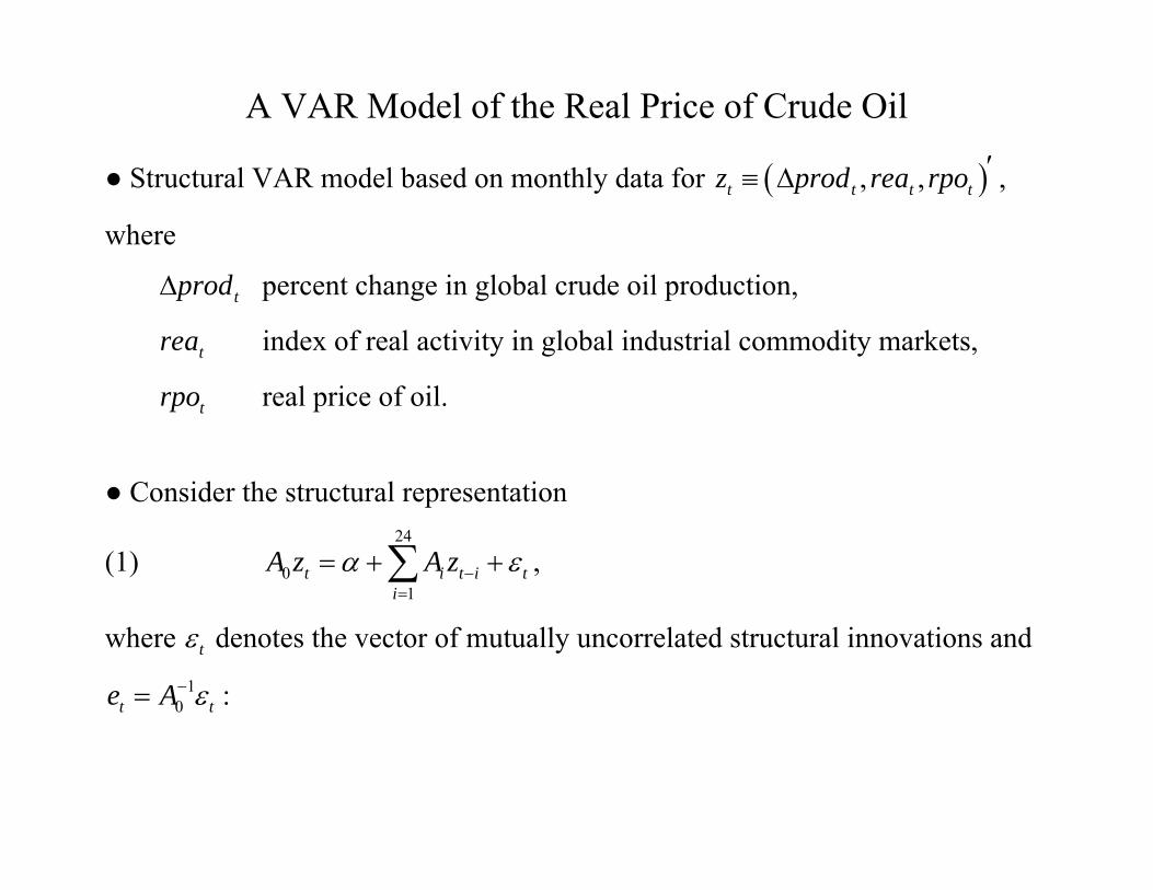
● Recent work by Kilian (2008) utilizes a structural VAR model of the global crude oil
market that addresses these three issues.
● This presentation will motivate and explain that approach to modeling oil markets and
highlight its implications for DSGE modeling.
Outline
1. The Determinants of the Real Price of Crude Oil
2. A Simple Structural Model of the Global Crude Oil Market
3. Understanding the Evolution of the Real Price of Oil Since 2000
4. The Transmission of Oil Demand and Oil Supply Shocks to the U.S.
Economy
5. Implications for DSGE Models of the Transmission of Oil Price Shocks
Part 1:
The Determinants of the Real Price of Crude Oil
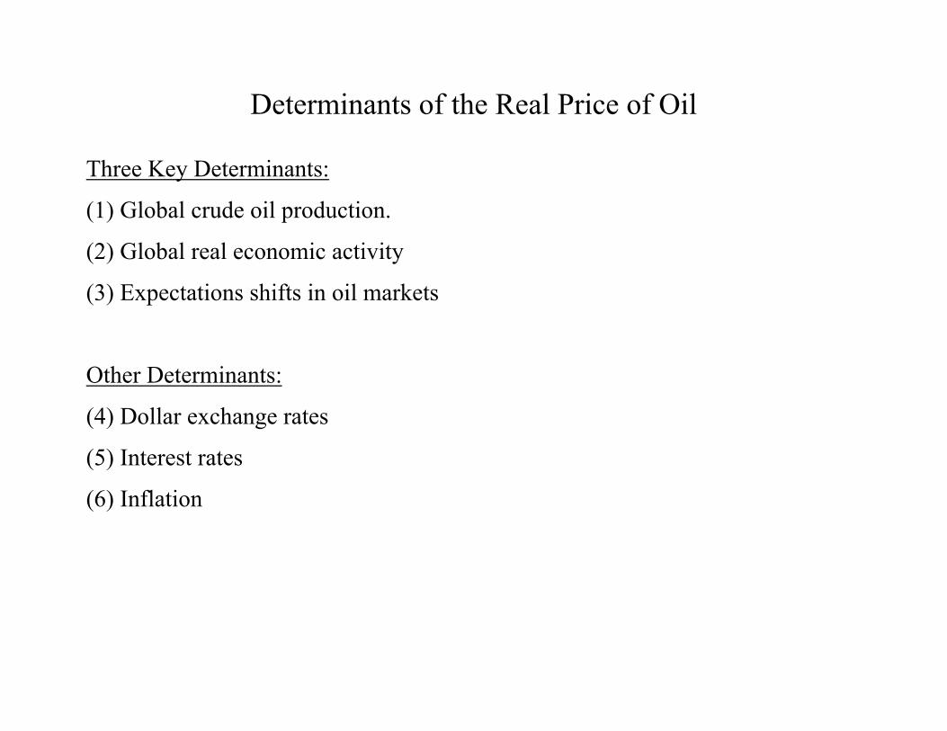
Determinants of the Real Price of Oil
Three Key Determinants:
(1) Global crude oil production.
(2) Global real economic activity
(3) Expectations shifts in oil markets
Other Determinants:
(4) Dollar exchange rates
(5) Interest rates
(6) Inflation
1975 1980 1985 1990 1995 2000 20050
10
20
30
40
50
60
70
80
90
100
Milli
ons
of B
arre
ls/D
ay
Crude Oil Production
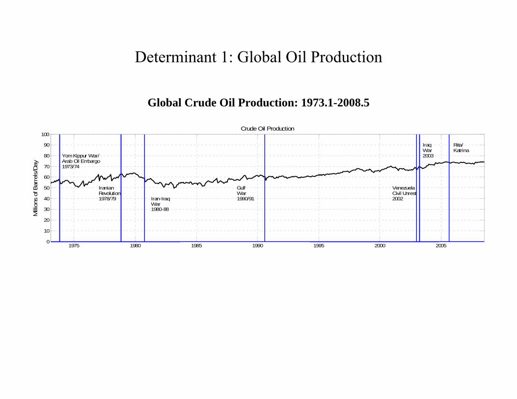
Yom Kippur War/Arab Oil Embargo1973/74
IranianRevolution1978/79 Iran-Iraq
War1980-88
GulfWar1990/91
VenezuelaCivil Unrest2002
IraqWar2003
Rita/Katrina
Determinant 1: Global Oil Production
Global Crude Oil Production: 1973.1-2008.5
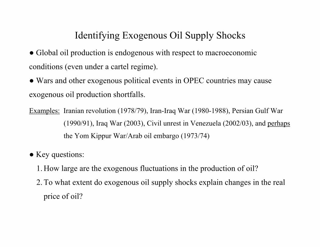
Identifying Exogenous Oil Supply Shocks
● Global oil production is endogenous with respect to macroeconomic
conditions (even under a cartel regime).
● Wars and other exogenous political events in OPEC countries may cause
exogenous oil production shortfalls.
Examples: Iranian revolution (1978/79), Iran-Iraq War (1980-1988), Persian Gulf War
(1990/91), Iraq War (2003), Civil unrest in Venezuela (2002/03), and perhaps
the Yom Kippur War/Arab oil embargo (1973/74)
● Key questions:
1. How large are the exogenous fluctuations in the production of oil?
2. To what extent do exogenous oil supply shocks explain changes in the real
price of oil?
Measuring Exogenous Oil Supply Shocks
● Hoover-Perez: Qualitative Dummies
● Hamilton (JoE 2003): Quantitative Dummies
● Kilian (REStat 2008): Any attempt to identify the timing and magnitude of
these exogenous production shortfalls requires explicit assumptions about the
counterfactual path of oil production in the absence of the exogenous event in
question.
Example: Counterfactual for the
October 1973 War and the 1973/74 Arab Oil Embargo
● It is well known that oil production from Arab OPEC countries fell between
September and November of 1973, whereas oil production in the rest of the
world did not.
● This observation suggests that we take non-OPEC oil producers as our
benchmark. Non-OPEC growth of oil production becomes the counterfactual.
● Simply comparing the production decisions in non-OPEC countries and Arab-
OPEC countries in late 1973 would be misleading, however, because of
differences in economic incentives across these countries.
1971 Tehran/Tripoli agreements
- Contract between the oil companies and Middle Eastern OPEC oil producers
- Duration of five years
- Moderate improvement in the financial terms that host governments receive from oil companies for each barrel of oil extracted by the oil companies …
… in exchange for assurances that these governments would allow the oil companies to extract as much oil as they saw fit on those terms.
● Latent problem: No allowance for excessive inflation or dollar devaluation ● Starting in early 1973 Arab OPEC oil producers complained of excessive oil
production.
● The agreements were unilaterally terminated by Middle Eastern OPEC in
early October of 1973, after unsuccessful attempts to renegotiate the terms in
response to the unanticipated dollar devaluation and high dollar inflation.
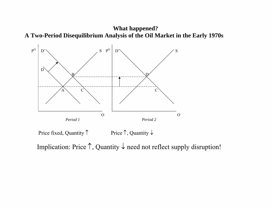
What happened? A Two-Period Disequilibrium Analysis of the Oil Market in the Early 1970s
Price fixed, Quantity ↑ Price ↑, Quantity ↓ Implication: Price ↑, Quantity ↓ need not reflect supply disruption!
O Period 2
O Period 1
D’ S PO D’ S D B D
A C C
PO
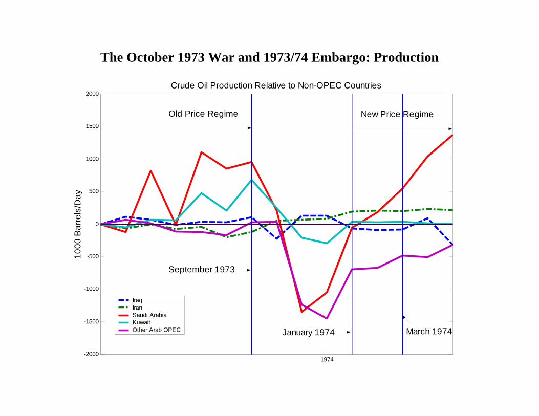
The October 1973 War and 1973/74 Embargo: Production
1974-2000
-1500
-1000
-500
0
500
1000
1500
2000Crude Oil Production Relative to Non-OPEC Countries
1000
Bar
rels
/Day
Old Price Regime New Price Regime
September 1973
January 1974 March 1974
Iraq Iran Saudi Arabia Kuwait Other Arab OPEC
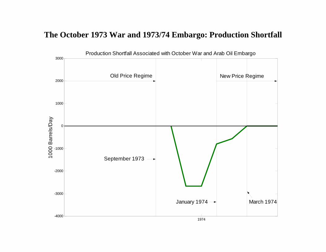
The October 1973 War and 1973/74 Embargo: Production Shortfall
1974-4000
-3000
-2000
-1000
0
1000
2000
3000Production Shortfall Associated with October War and Arab Oil Embargo
1000
Bar
rels
/Day
Old Price Regime New Price Regime
September 1973
March 1974January 1974
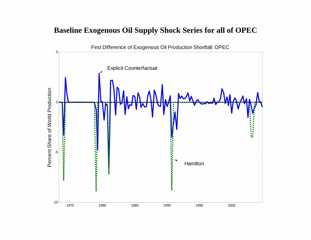
Baseline Exogenous Oil Supply Shock Series for all of OPEC
1975 1980 1985 1990 1995 2000-10
-5
0
5First Difference of Exogenous Oil Production Shortfall: OPEC
Per
cent
Sha
re o
f Wor
ld P
rodu
ctio
n
Explicit Counterfactual
Hamilton
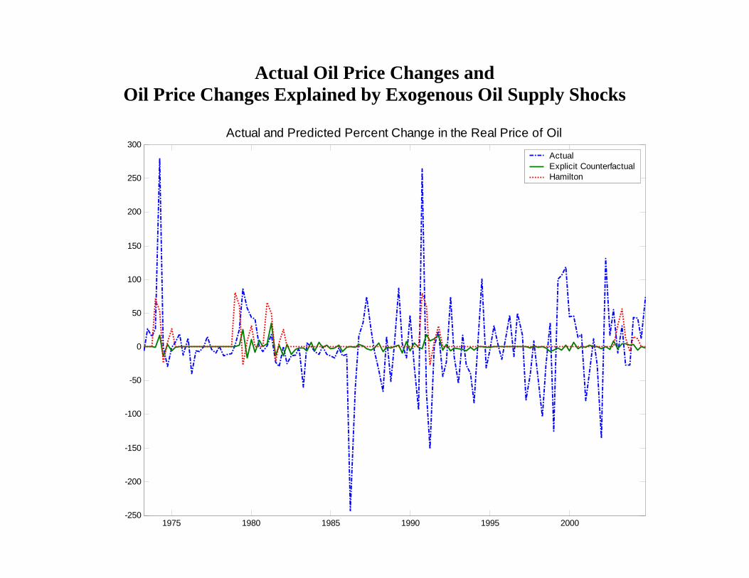
Actual Oil Price Changes and Oil Price Changes Explained by Exogenous Oil Supply Shocks
1975 1980 1985 1990 1995 2000-250
-200
-150
-100
-50
0
50
100
150
200
250
300Actual and Predicted Percent Change in the Real Price of Oil
Actual Explicit CounterfactualHamilton
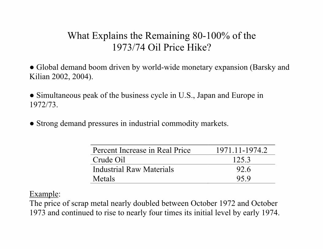
What Explains the Remaining 80-100% of the 1973/74 Oil Price Hike?
● Global demand boom driven by world-wide monetary expansion (Barsky and Kilian 2002, 2004). ● Simultaneous peak of the business cycle in U.S., Japan and Europe in 1972/73. ● Strong demand pressures in industrial commodity markets.
Percent Increase in Real Price 1971.11-1974.2 Crude Oil 125.3 Industrial Raw Materials 92.6 Metals 95.9
Example: The price of scrap metal nearly doubled between October 1972 and October 1973 and continued to rise to nearly four times its initial level by early 1974.
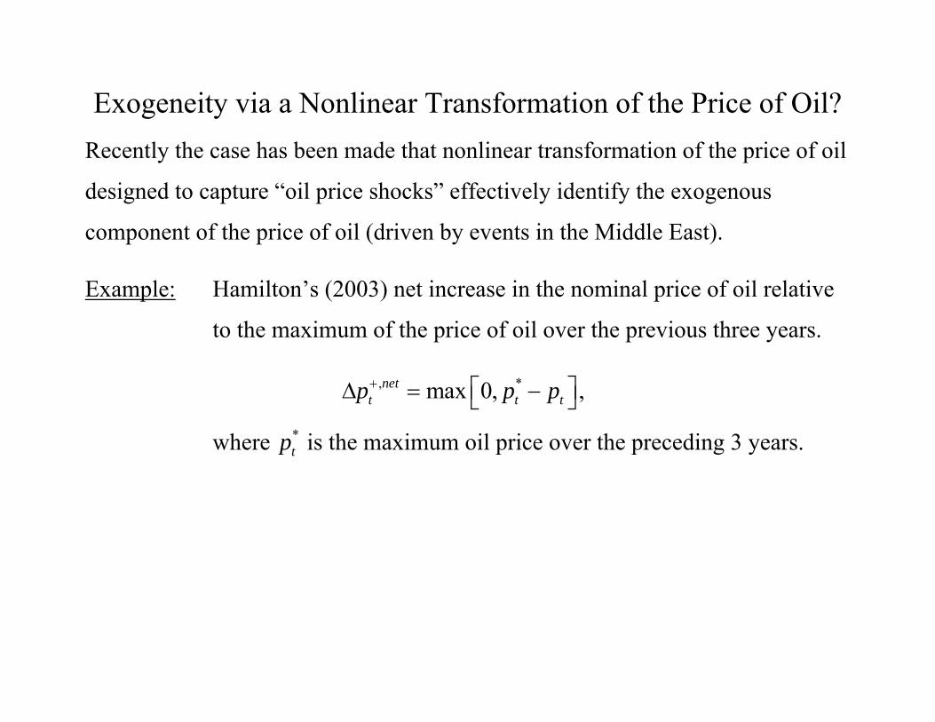
Exogeneity via a Nonlinear Transformation of the Price of Oil? Recently the case has been made that nonlinear transformation of the price of oil
designed to capture “oil price shocks” effectively identify the exogenous
component of the price of oil (driven by events in the Middle East).
Example: Hamilton’s (2003) net increase in the nominal price of oil relative
to the maximum of the price of oil over the previous three years.
, *max 0,nett t tp p p+ ⎡ ⎤Δ = −⎣ ⎦ ,
where *tp is the maximum oil price over the preceding 3 years.
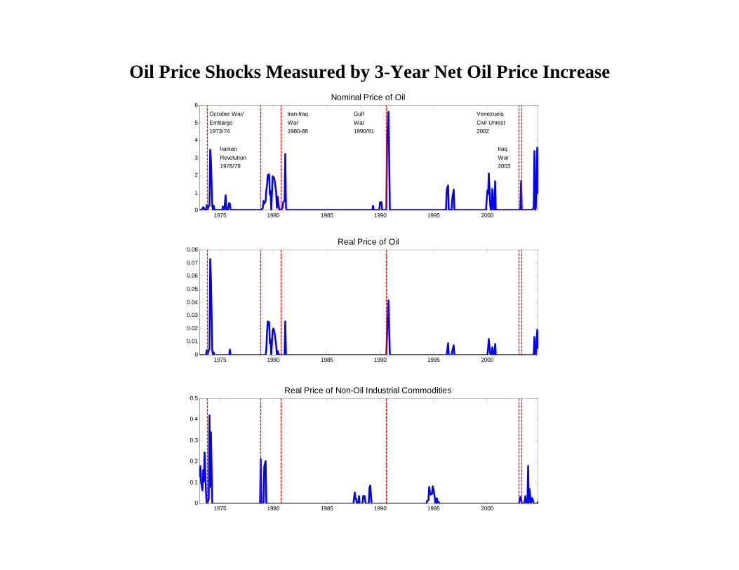
Oil Price Shocks Measured by 3-Year Net Oil Price Increase
1975 1980 1985 1990 1995 20000
1
2
3
4
5
6Nominal Price of Oil
October War/Embargo1973/74
IranianRevolution1978/79
Iran-IraqWar1980-88
GulfWar1990/91
VenezuelaCivil Unrest2002
IraqWar2003
1975 1980 1985 1990 1995 20000
0.01
0.02
0.03
0.04
0.05
0.06
0.07
0.08Real Price of Oil
1975 1980 1985 1990 1995 20000
0.1
0.2
0.3
0.4
0.5Real Price of Non-Oil Industrial Commodities
● Clearly, the net increase measure is not exogenous with respect to
macroeconomic conditions (previous evidence to the contrary has been
inadmissible).
● The recent literature has instead treated the net increase measure as
predetermined with respect to the domestic macro economy:
,
~ ( )net
t
t
pVAR p
y
+⎛ ⎞Δ⎜ ⎟⎝ ⎠
Kilian and Vigfusson (2009) show that such regressions are inherently
mispecified, the parameter estimates are inconsistent, and the impulse response
estimates have been computed incorrectly, resulting in response estimates that
are typically upward biased.
● Moreover, there is no formal evidence supporting this type of model of the
transmission of oil price shocks.
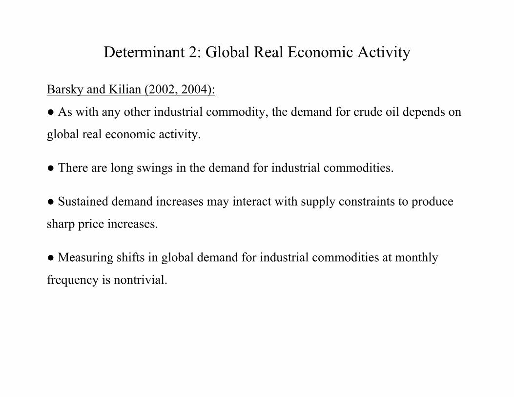
Determinant 2: Global Real Economic Activity
Barsky and Kilian (2002, 2004):
● As with any other industrial commodity, the demand for crude oil depends on
global real economic activity.
● There are long swings in the demand for industrial commodities.
● Sustained demand increases may interact with supply constraints to produce
sharp price increases.
● Measuring shifts in global demand for industrial commodities at monthly
frequency is nontrivial.
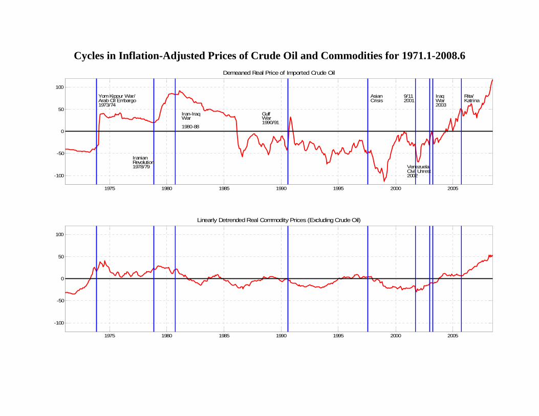
1975 1980 1985 1990 1995 2000 2005
-100
-50
0
50
100
Demeaned Real Price of Imported Crude Oil
Yom Kippur War/Arab Oil Embargo1973/74
IranianRevolution1978/79
Iran-IraqWar
1980-88
GulfWar1990/91
AsianCrisis
9/112001
Rita/Katrina
VenezuelaCivil Unrest2002
IraqWar2003
1975 1980 1985 1990 1995 2000 2005
-100
-50
0
50
100
Linearly Detrended Real Commodity Prices (Excluding Crude Oil)
Cycles in Inflation-Adjusted Prices of Crude Oil and Commodities for 1971.1-2008.6
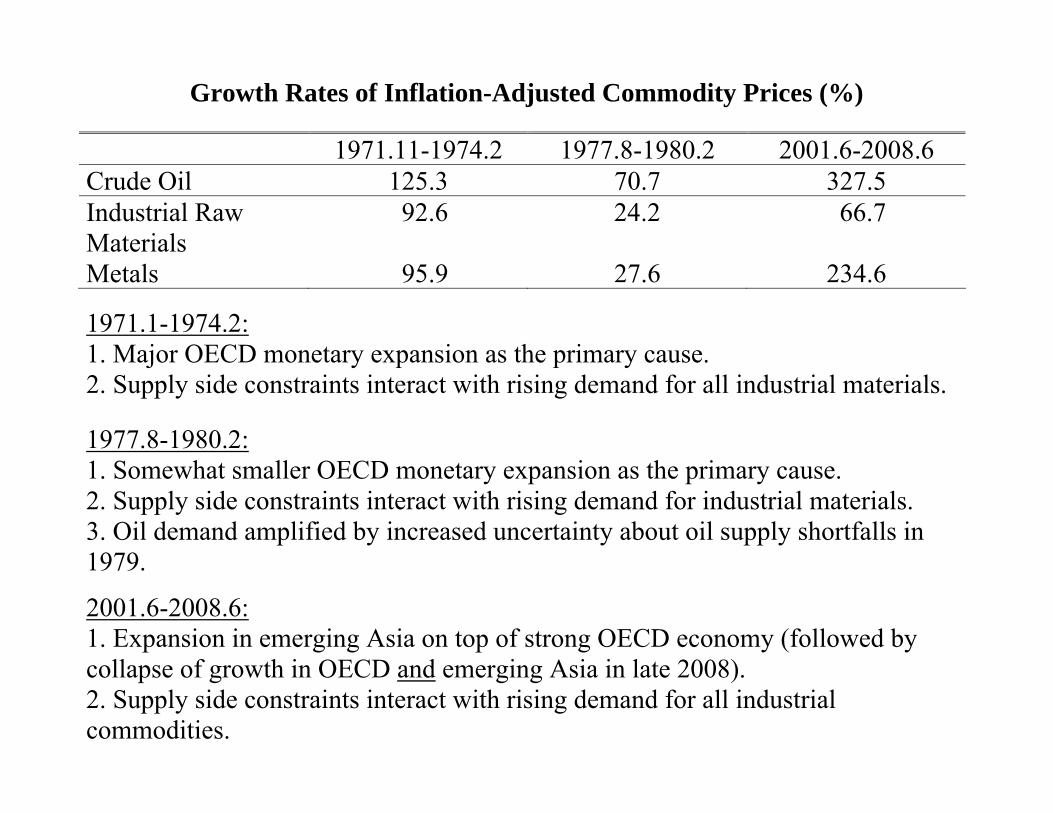
Growth Rates of Inflation-Adjusted Commodity Prices (%)
1971.1-1974.2: 1. Major OECD monetary expansion as the primary cause. 2. Supply side constraints interact with rising demand for all industrial materials.
1977.8-1980.2: 1. Somewhat smaller OECD monetary expansion as the primary cause. 2. Supply side constraints interact with rising demand for industrial materials. 3. Oil demand amplified by increased uncertainty about oil supply shortfalls in 1979.
2001.6-2008.6: 1. Expansion in emerging Asia on top of strong OECD economy (followed by collapse of growth in OECD and emerging Asia in late 2008). 2. Supply side constraints interact with rising demand for all industrial commodities.
A Monthly Index of Global Real Activity based on
Ocean Shipping Freight Rates
● Based on representative ocean shipping freight rates collected by Drewry Shipping
Consultants Ltd. for various bulk dry cargoes including grain, oilseeds, coal, iron ore,
fertilizer and scrap metal.
● Available at monthly frequency as far back as January 1968.
● Not without precedence:
1. Economists have long observed a positive correlation between ocean freight rates
2. It is widely accepted that world economic activity is by far the most important
determinant of the demand for transport services (see, e.g., Klovland 2004).
3. The same approach is used by market practitioners (Baltic Dry Cargo Index).
How Freight Rates Reflect Real Economic Activity
● At low levels of freight volumes the supply curve of shipping is relatively flat in the
short and intermediate run, as idle ships may be reactivated or active ships may simply
cut short layovers and run faster.
● As the demand schedule for shipping services shifts out due to increased economic
activity, the slope of the supply curve becomes increasingly steeper and freight rates
increase. At full capacity the supply curve becomes effectively vertical, as all available
ships are operational and running at full speed.
● This line of reasoning suggests that net increases in freight rates relative to the recent
past may be used as indicators of strong cumulative global demand pressures.
Disadvantages and Advantages of the Proposed Index
Disadvantages:
The presence of a ship-building and scrapping cycle may weaken the business cycle in
global commodity markets and the freight rate index.
Given the pro-cyclicality of ship-building, one would expect the real freight rate index to
lag increases in real economic activity (as spare capacity in shipping cushions the impact
of higher demand on freight rates) and to lead decreases in real economic activity (as the
arrival of new ships depresses freight rates), thus accentuating upswings in real activity.
Advantages:
The proposed index is a direct measure of global economic activity that (1) does not
require exchange-rate weighting, that (2) automatically aggregates real economic activity
in all countries (including, e.g., China, India), and that (3) already incorporates shifting
country weights, changes in the composition of real output, and changes in the propensity
to import industrial commodities for a given unit of real output.
Construction of the Index in Practice
● Single voyage freight rates
● Only bulk dry cargoes (no substitutability)
● Freight rates are typically quoted in U.S. dollars per metric ton.
● Monthly quotes are provided for different commodities, routes and ship sizes.
● There is no continuous series for the entire sample period.
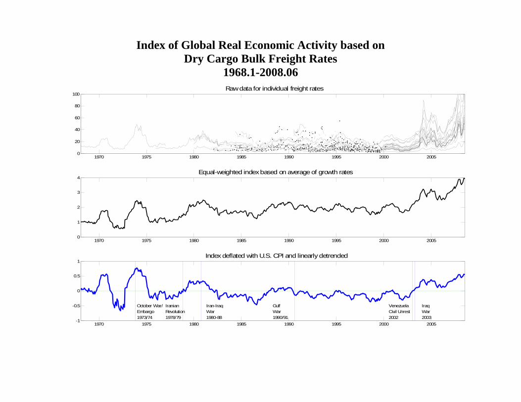
1970 1975 1980 1985 1990 1995 2000 20050
20
40
60
80
100Raw data for individual freight rates
1970 1975 1980 1985 1990 1995 2000 20050
1
2
3
4Equal-weighted index based on average of growth rates
1970 1975 1980 1985 1990 1995 2000 2005-1
-0.5
0
0.5
1
October War/Embargo1973/74
IranianRevolution1978/79
Iran-IraqWar1980-88
GulfWar1990/91
VenezuelaCivil Unrest2002
IraqWar2003
Index deflated with U.S. CPI and linearly detrended
Index of Global Real Economic Activity based on Dry Cargo Bulk Freight Rates
1968.1-2008.06
Rationale of the Proposed Index (1) ● A concern is that dry cargo freight rates may increase during oil price shocks
not because both are driven by higher demand for commodities, but because the
provision of shipping services uses bunker fuel oil as an input.
Response:
1. The model below used for the empirical analysis allows for unrestricted
lagged feedback from oil prices to freight rates.
2. Data on the real price of bunker fuel from the Oil and Gas Journal are
consistent with that assumption.
1970.5 1971 1971.5 1972 1972.5 1973 1973.5 1974-1
-0.8
-0.6
-0.4
-0.2
0
0.2
0.4
0.6
0.8
1
Real economic activityBunker Fuel Rates
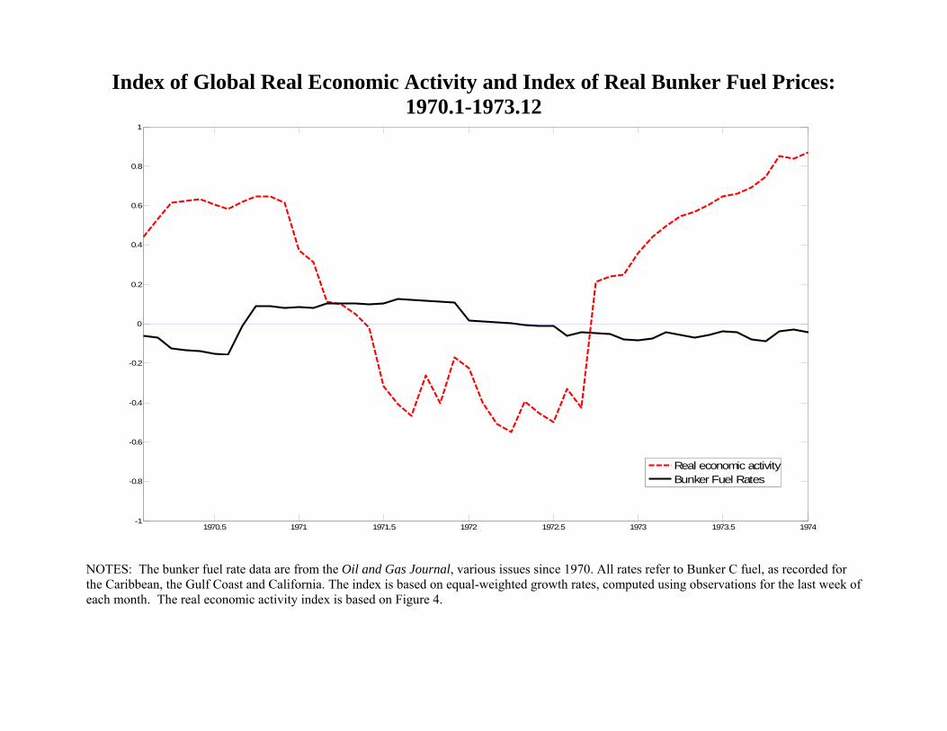
Index of Global Real Economic Activity and Index of Real Bunker Fuel Prices: 1970.1-1973.12
NOTES: The bunker fuel rate data are from the Oil and Gas Journal, various issues since 1970. All rates refer to Bunker C fuel, as recorded for the Caribbean, the Gulf Coast and California. The index is based on equal-weighted growth rates, computed using observations for the last week of each month. The real economic activity index is based on Figure 4.
Rationale of the Proposed Index (2)
● Why not include data on crude oil tanker rates available from Drewry’s
Shipping Monthly?
Response: Typically these rates strongly co-move with dry cargo rates, but tanker rates at times may
be subject to important oil-specific supply shocks, which makes them unsuitable as a
measure of real economic activity:
(1) Events such an oil embargo may lower the demand for tankers (and hence tanker
rates) simply because there is no oil to be shipped, not because consumers’ demand for
oil has decreased.
(2) Attacks on shipping in the Persian Gulf may raise the insurance premium for tankers
(and hence tanker rates). The same applies to transportation surcharges, as tankers are
rerouted.
Rationale of the Proposed Index (3)
● Alternative Measures:
1. The Baltic Dry Cargo Index (available since 1985) is essentially identical
with the freight rate index underlying the proposed measure of global
real activity.
2. Monthly Index of Global Industrial Production?
- No world industrial production available at monthly frequency
- OECD industrial production excludes many emerging economies in Asia
and misses the demand boom from emerging economies.
Lesson: We need a truly global measure of real activity.
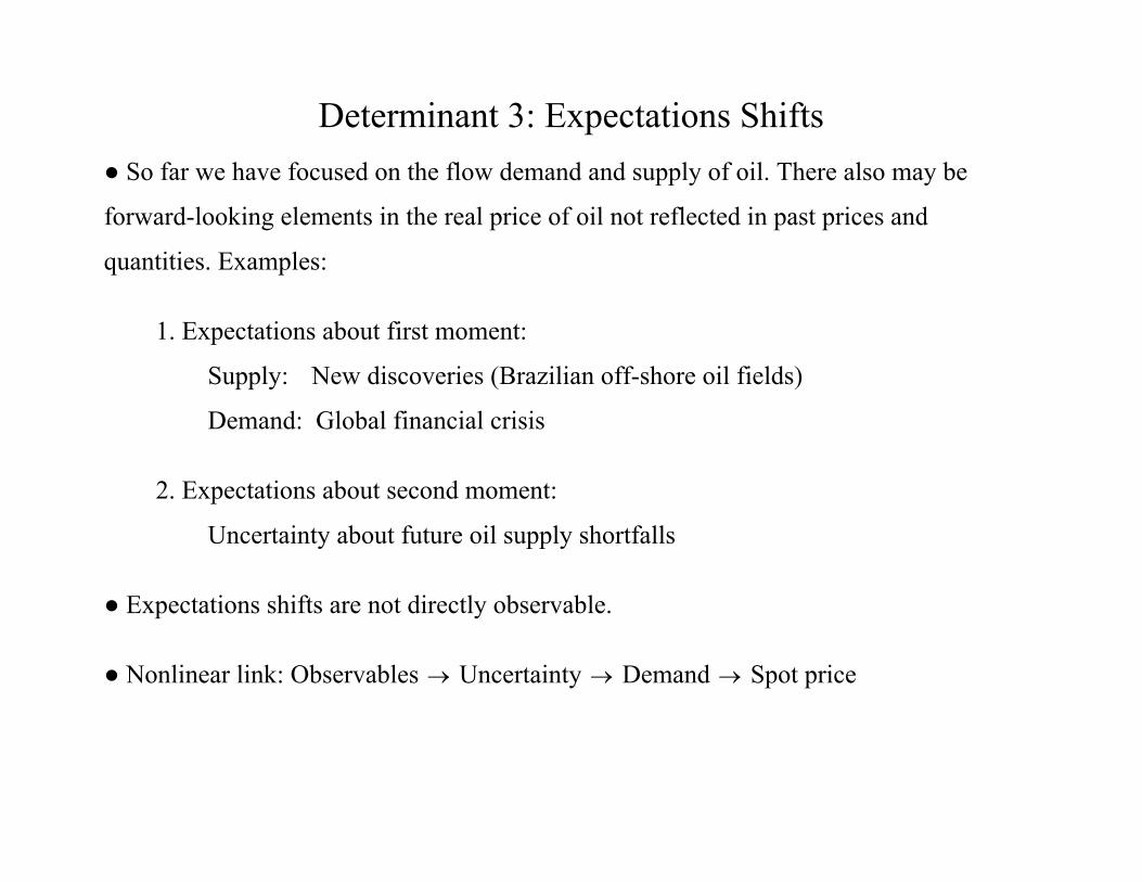
Determinant 3: Expectations Shifts ● So far we have focused on the flow demand and supply of oil. There also may be
forward-looking elements in the real price of oil not reflected in past prices and
quantities. Examples:
1. Expectations about first moment:
Supply: New discoveries (Brazilian off-shore oil fields)
Demand: Global financial crisis
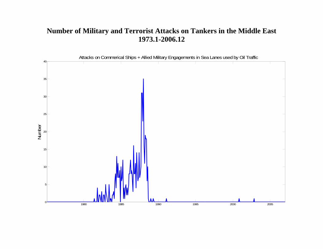
2. Expectations about second moment:
Uncertainty about future oil supply shortfalls
● Expectations shifts are not directly observable.
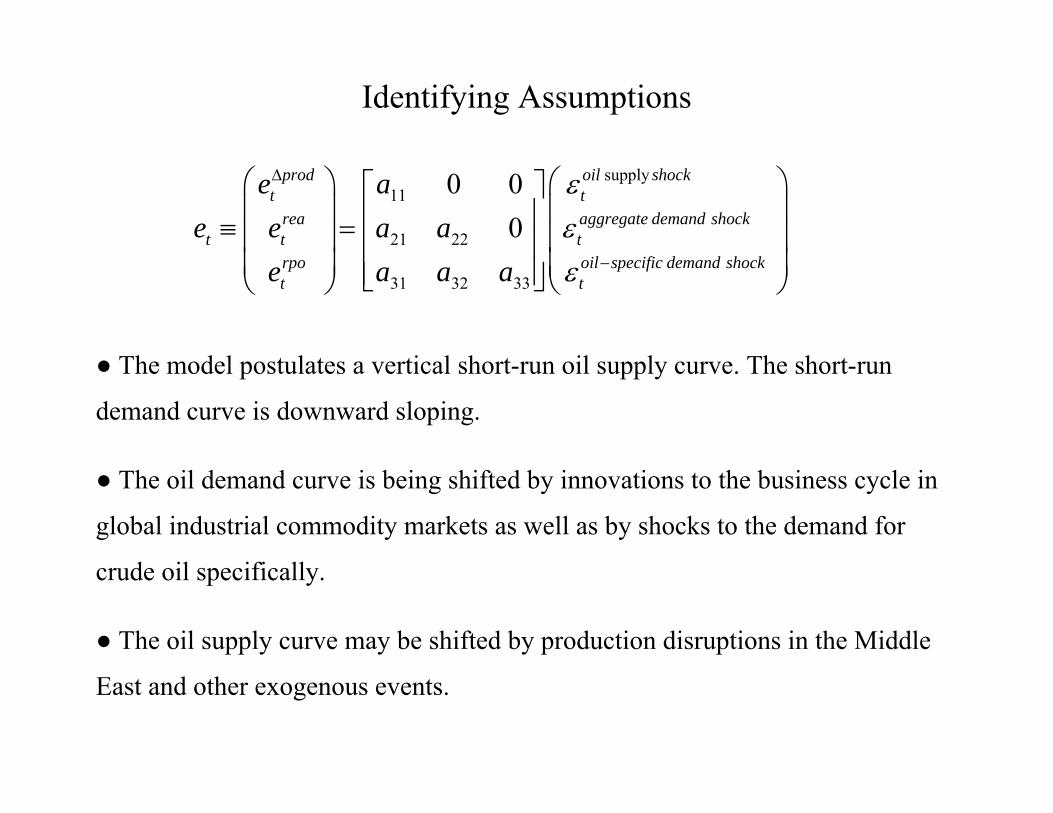
● The model postulates a vertical short-run oil supply curve. The short-run
demand curve is downward sloping.
● The oil demand curve is being shifted by innovations to the business cycle in
global industrial commodity markets as well as by shocks to the demand for
crude oil specifically.
● The oil supply curve may be shifted by production disruptions in the Middle
East and other exogenous events.
Evidence in Support of the Exclusion Restrictions
● Changing supply is costly.
● Supply decisions depend on expected demand growth:
- AARAMCO model of oil demand only updated once a year.
- Evidence that OPEC was slow to respond to world recession in early 1980s.
● Oil-specific demand does not affect business cycle in global commodity
markets within a month:
- Plausible given delayed reaction of OECD economies to oil price shocks.
1976 1977 1978 1979 1980 1981 1982 1983-1
-0.5
0
0.5
1Oil Supply Shock
1976 1977 1978 1979 1980 1981 1982 1983-1
-0.5
0
0.5
1Aggregate Demand Shock
1976 1977 1978 1979 1980 1981 1982 1983-1
-0.5
0
0.5
1Oil-Specific Demand Shock
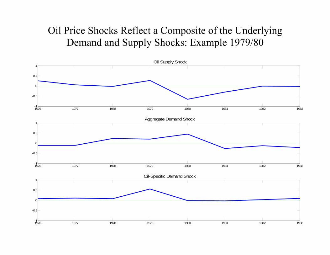
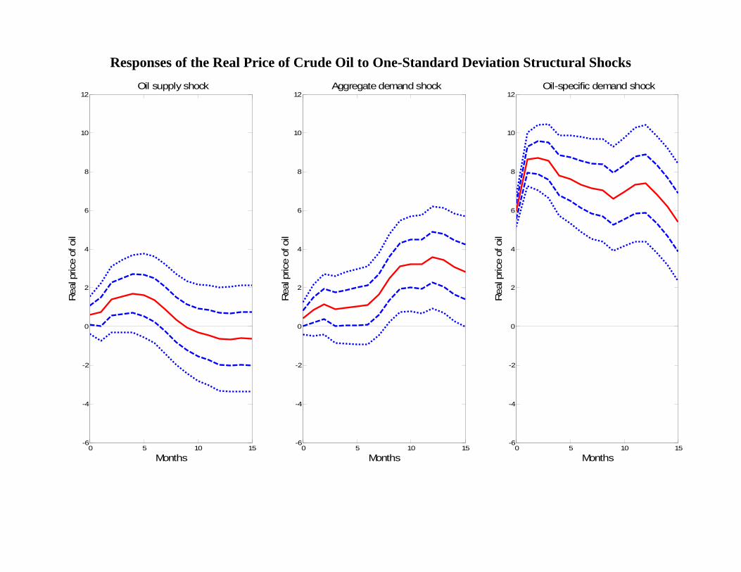
Oil Price Shocks Reflect a Composite of the Underlying Demand and Supply Shocks: Example 1979/80
0 5 10 15-6
-4
-2
0
2
4
6
8
10
12Oil supply shock
Rea
l pric
e of
oil
Months0 5 10 15
-6
-4
-2
0
2
4
6
8
10
12Aggregate demand shock
Rea
l pric
e of
oil
Months0 5 10 15
-6
-4
-2
0
2
4
6
8
10
12Oil-specific demand shock
Rea
l pric
e of
oil
Months
Responses of the Real Price of Crude Oil to One-Standard Deviation Structural Shocks
1980 1985 1990 1995 2000 2005-100
-50
0
50
100Cumulative Effect of Global Oil Supply Shock on Real Price of Crude Oil
1980 1985 1990 1995 2000 2005-100
-50
0
50
100Cumulative Effect of Global Aggregate Demand Shock on Real Price of Crude Oil
1980 1985 1990 1995 2000 2005-100
-50
0
50
100Cumulative Effect of Oil-Market Specific Demand Shock on Real Price of Crude Oil
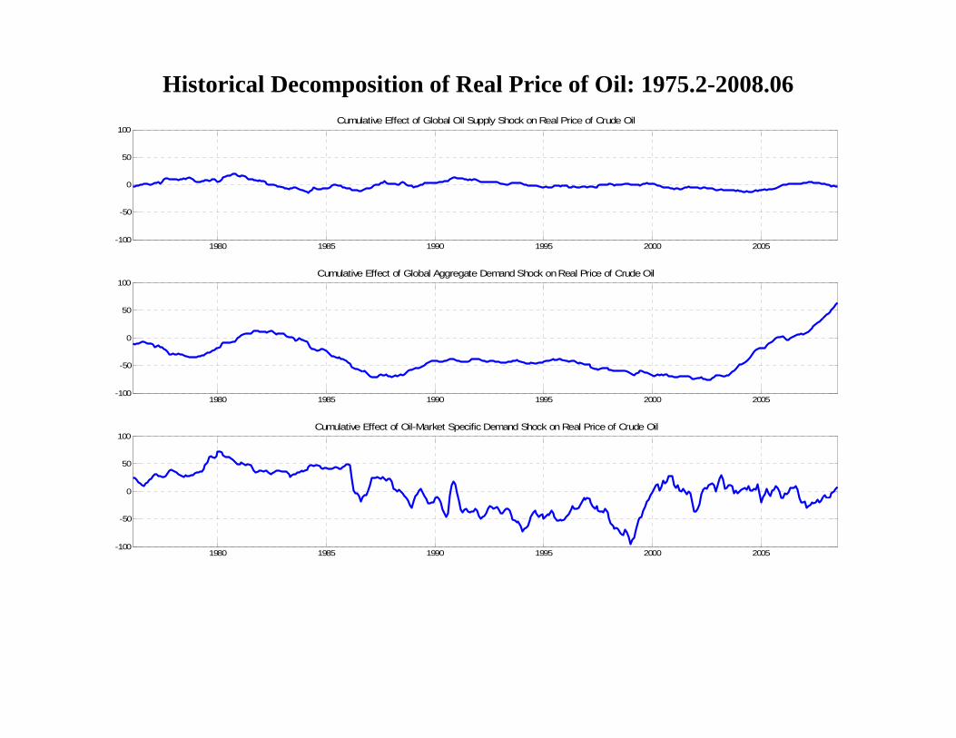
Historical Decomposition of Real Price of Oil: 1975.2-2008.06
Rationale for Interpreting Oil-Specific Demand Shocks as
Precautionary Demand Shocks
● No other plausible candidates (e.g., notion of disproportionately increased preference
for oil in China in recent years is inconsistent with VAR evidence).
● The timing of these shocks is consistent with the timing of events that should trigger
shifts in precautionary demand.
● Alquist and Kilian (2008) use data on oil futures prices to identify an index of the
precautionary demand component of the real price of oil for 1989-2007, which is highly
correlated with the VAR-based measure.
1990 1992 1994 1996 1998 2000 2002 2004 2006-100
-80
-60
-40
-20
0
20
40
60
80
100
Negative Basis at 12-Month HorizonVAR-Based Precautionary Demand Component of Spot Price
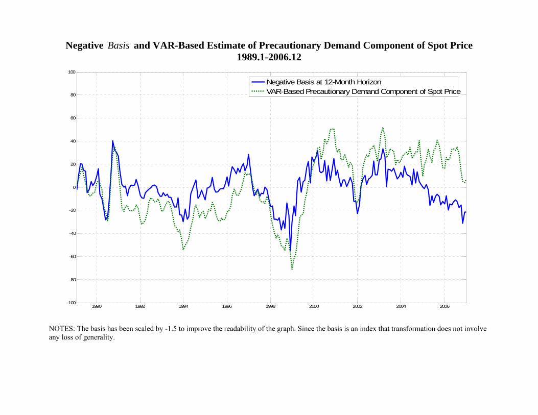
Negative Basis and VAR-Based Estimate of Precautionary Demand Component of Spot Price 1989.1-2006.12
NOTES: The basis has been scaled by -1.5 to improve the readability of the graph. Since the basis is an index that transformation does not involve any loss of generality.
Part 3:
Understanding the Evolution of the Real Price of Oil Since 2000
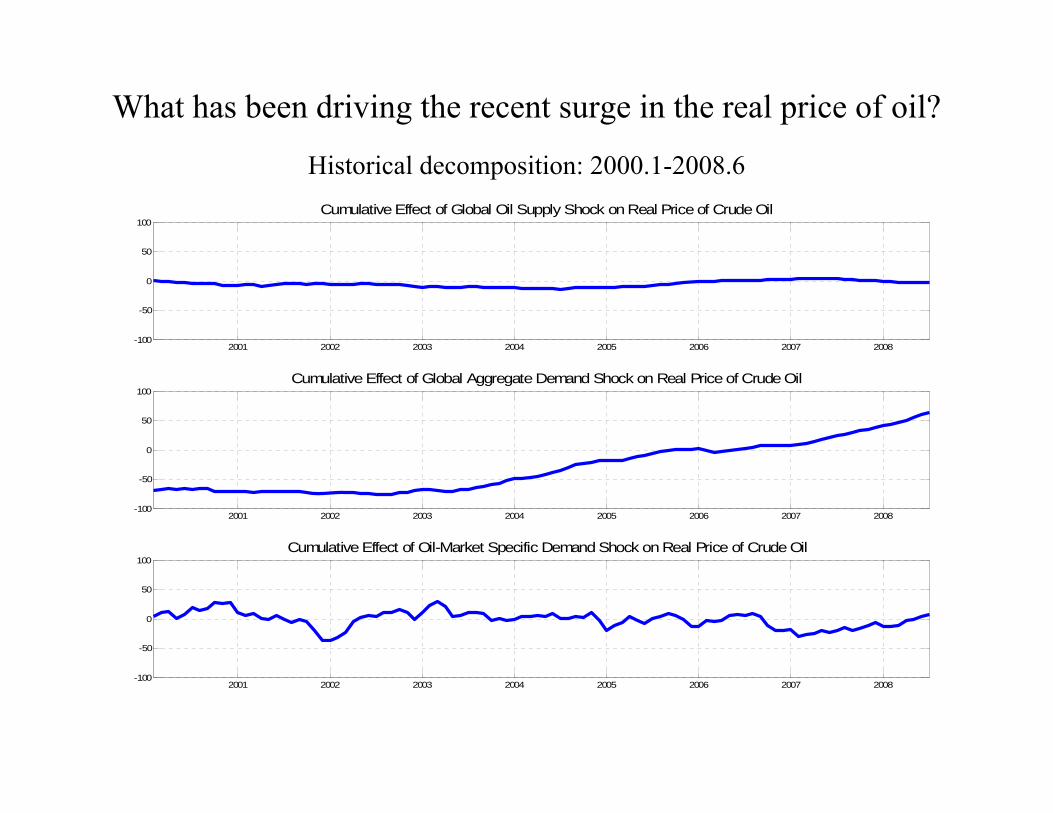
2001 2002 2003 2004 2005 2006 2007 2008-100
-50
0
50
100Cumulative Effect of Global Oil Supply Shock on Real Price of Crude Oil
2001 2002 2003 2004 2005 2006 2007 2008-100
-50
0
50
100Cumulative Effect of Global Aggregate Demand Shock on Real Price of Crude Oil
2001 2002 2003 2004 2005 2006 2007 2008-100
-50
0
50
100Cumulative Effect of Oil-Market Specific Demand Shock on Real Price of Crude Oil
What has been driving the recent surge in the real price of oil?
Historical decomposition: 2000.1-2008.6
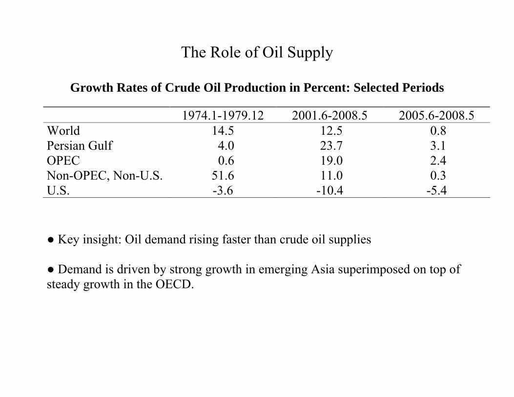
The Role of Oil Supply
Growth Rates of Crude Oil Production in Percent: Selected Periods
1974.1-1979.12 2001.6-2008.5 2005.6-2008.5 World 14.5 12.5 0.8 Persian Gulf 4.0 23.7 3.1 OPEC 0.6 19.0 2.4 Non-OPEC, Non-U.S. 51.6 11.0 0.3 U.S. -3.6 -10.4 -5.4
● Key insight: Oil demand rising faster than crude oil supplies ● Demand is driven by strong growth in emerging Asia superimposed on top of steady growth in the OECD.
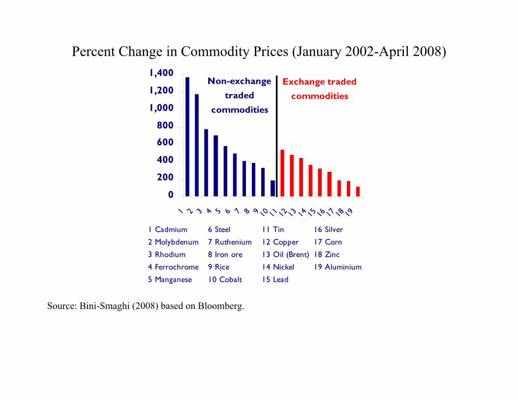
Alternative 1: Has the recent surge been driven by speculation? ● Speculation could not have been oil market specific or the econometric model would have picked it up as an oil-specific demand shock. ● This leaves the possibility of futures-market driven speculation in many industrial commodity markets. Problem:
Industrial commodity prices rose similarly in markets for which no futures contracts exist.
0
200
400
600
800
1,000
1,200
1,400
1 2 3 4 5 6 7 8 9 10 11 12 13 14 15 16 17 18 19
Exchange traded commodities
Non-exchange traded
commodities
1 Cadmium
2 Molybdenum
3 Rhodium
4 Ferrochrome
5 Manganese
6 Steel
7 Ruthenium
8 Iron ore
9 Rice
10 Cobalt
11 Tin
12 Copper
13 Oil (Brent)
14 Nickel
15 Lead
16 Silver
17 Corn
18 Zinc
19 Aluminium
Percent Change in Commodity Prices (January 2002-April 2008) Source: Bini-Smaghi (2008) based on Bloomberg.
● There was an increase in share of “speculators” in oil futures markets in 2003. ● Suppose that speculators drive up oil futures prices. Why would this matter? If higher oil futures prices are interpreted as a prediction of higher spot prices,
spot traders will buy a barrel of oil and store it with the intention of selling it a
year later at a higher price and making a profit.
Problems with this explanation:
1. Evidence suggests that speculators played both sides of the futures markets
rather than consistently betting on higher prices.
2. Alquist and Kilian (2008) have shown that oil futures prices are no better
predictors of the spot price than no-change forecasts.
3. Suppose, nevertheless, that spot market traders acted as though oil futures prices
predict spot prices:
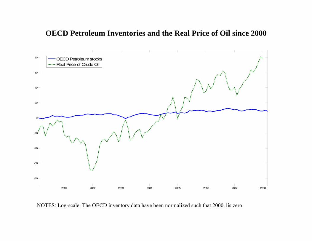
a. In that case, according to standard economic models, one would expect above-ground oil inventories to have increased sharply relative to trend since 2003. Problem: That did not occur in the U.S. and OECD data. CAVEAT: Not all above-ground oil inventories are monitored adequately.
2001 2002 2003 2004 2005 2006 2007 2008
-80
-60
-40
-20
0
20
40
60
80 OECD Petroleum stocksReal Price of Crude Oil
OECD Petroleum Inventories and the Real Price of Oil since 2000 NOTES: Log-scale. The OECD inventory data have been normalized such that 2000.1is zero.
b. If, for technological reasons, the stock of oil in inventories is fixed, increased speculation in the spot market means that traditional buyers must have received less crude oil. Problem: Those traditional buyers are refineries, so their output in the form of gasoline, heating oil, etc. should have fallen since 2003. This again is inconsistent with the data.
Alternative 2: Is U.S. monetary policy to blame?
Expansionary monetary policy played central role in oil price increases (and
declines) of the 1970s and early 1980s. It did not play a key role in the
2000s:
● Openly stimulative U.S. policy only as of late. Can’t explain past oil price increases since 2001.
● U.S. monetary expansion since 2001 tempered by concerns about financial stability. Inflation expectations remained anchored.
● No similar monetary expansion elsewhere in the OECD.
● Recent oil price boom driven by emerging Asia rather than the OECD.
● Quantitative importance of the weakening dollar for the demand for oil (and the extent to which it depends on monetary policy) is unclear.
1975 1980 1985 1990 1995 2000 2005
-60
-40
-20
0
20
40
60
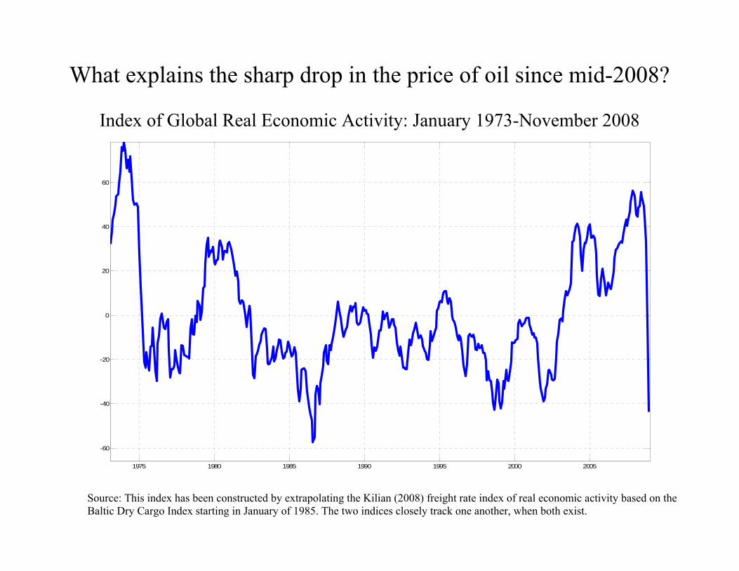
What explains the sharp drop in the price of oil since mid-2008?
Index of Global Real Economic Activity: January 1973-November 2008 Source: This index has been constructed by extrapolating the Kilian (2008) freight rate index of real economic activity based on the Baltic Dry Cargo Index starting in January of 1985. The two indices closely track one another, when both exist.
1980 1985 1990 1995 2000 2005 2010-100
-80
-60
-40
-20
0
20
40
60
80
100Cumulative Effect of Global Aggregate Demand Shock on Global Real Activity
1980 1985 1990 1995 2000 2005 2010-100
-80
-60
-40
-20
0
20
40
60
80
100Cumulative Effect of Global Aggregate Demand Shock on Real Price of Crude Oil
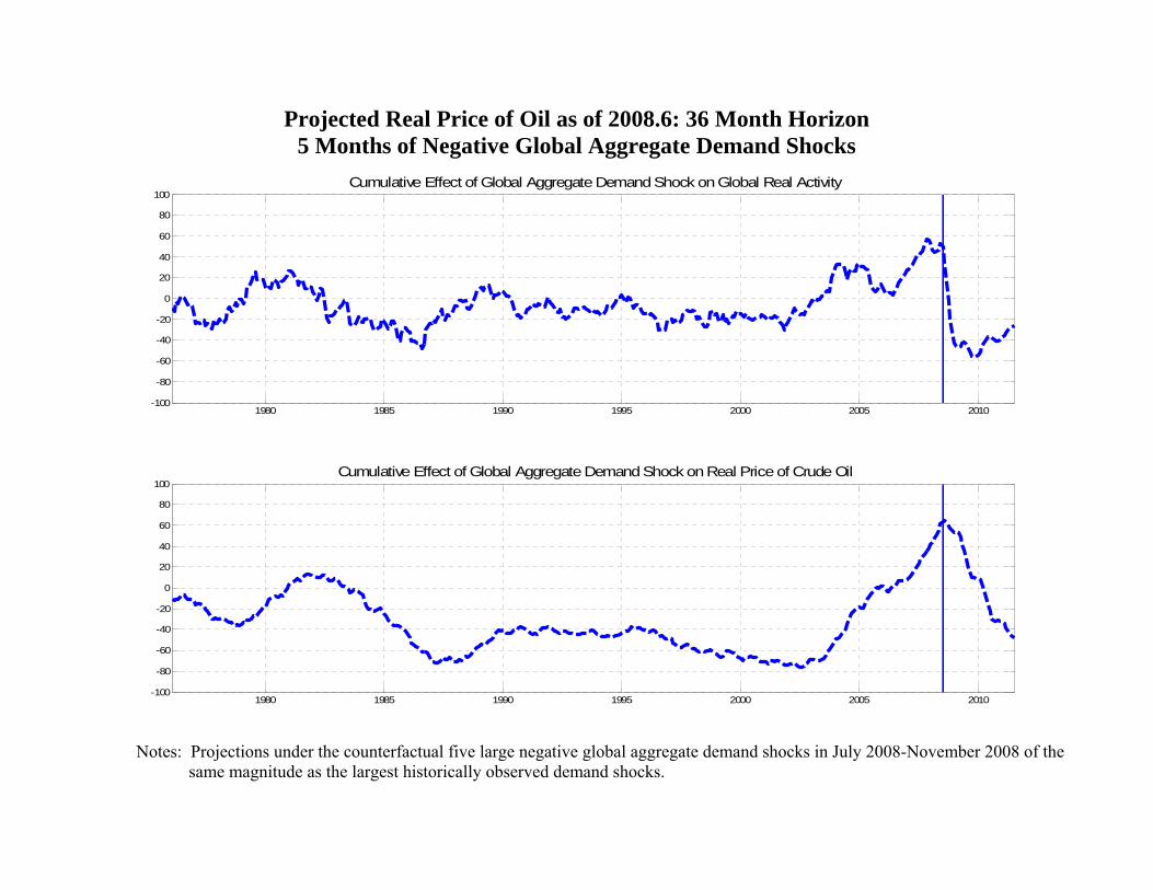
Projected Real Price of Oil as of 2008.6: 36 Month Horizon 5 Months of Negative Global Aggregate Demand Shocks
Notes: Projections under the counterfactual five large negative global aggregate demand shocks in July 2008-November 2008 of the same magnitude as the largest historically observed demand shocks.
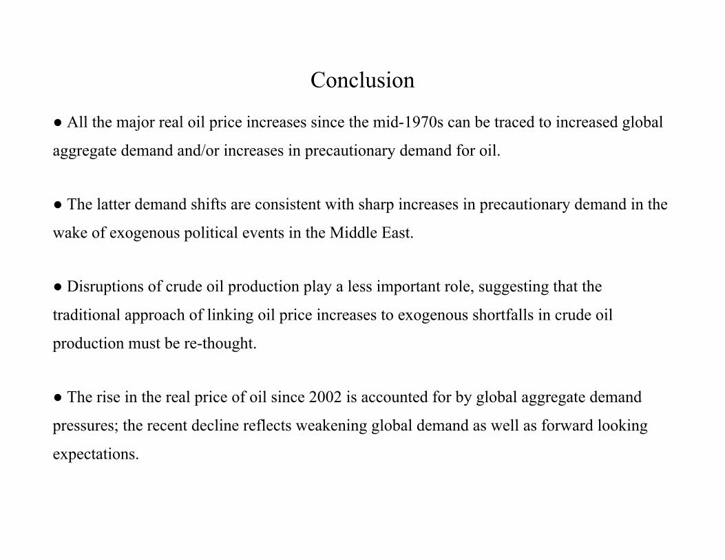
Conclusion
● All the major real oil price increases since the mid-1970s can be traced to increased global
aggregate demand and/or increases in precautionary demand for oil.
● The latter demand shifts are consistent with sharp increases in precautionary demand in the
wake of exogenous political events in the Middle East.
● Disruptions of crude oil production play a less important role, suggesting that the
traditional approach of linking oil price increases to exogenous shortfalls in crude oil
production must be re-thought.
● The rise in the real price of oil since 2002 is accounted for by global aggregate demand
pressures; the recent decline reflects weakening global demand as well as forward looking
expectations.
Part 4:
The Transmission of Oil Demand and Oil Supply Shocks to the U.S. Economy
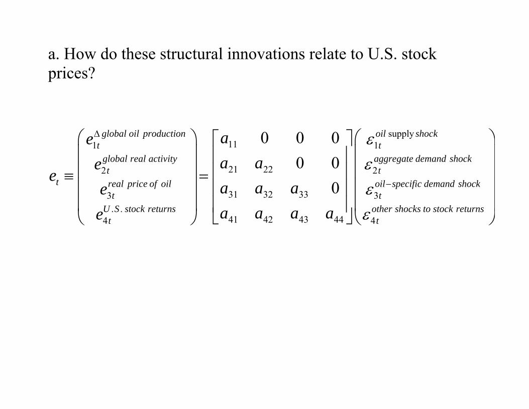
a. How do these structural innovations relate to U.S. stock prices?
supply
111 1
21 222 2
31 32 333 3. .
41 42 43 444
0 0 00 0
0
global oil production oil shockt t
global real activity aggregate demand shockt t
t real price of oil oil specific dt t
U S stock returnst
aea ae
ea a aea a a ae
εεε
Δ
−
⎛ ⎞ ⎡ ⎤⎜ ⎟ ⎢ ⎥⎜ ⎟ ⎢ ⎥≡ =⎜ ⎟ ⎢ ⎥⎜ ⎟ ⎢ ⎥
⎣ ⎦⎝ ⎠ 4
emand shock
other shocks to stock returnstε
⎛ ⎞⎜ ⎟⎜ ⎟⎜ ⎟⎜ ⎟⎝ ⎠
0 5 10−4
−3
−2
−1
0
1
2
3
4
Months
Per
cent
Oil Supply Shock
0 5 10−4
−3
−2
−1
0
1
2
3
4
Months
Per
cent
Aggregate Demand Shock
0 5 10−4
−3
−2
−1
0
1
2
3
4
Months
Per
cent
Oil−Market Specific Demand Shock
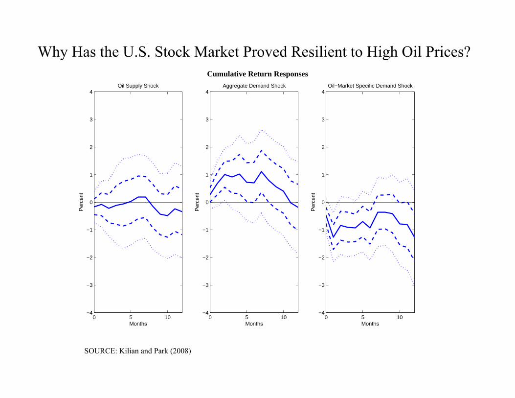
Why Has the U.S. Stock Market Proved Resilient to High Oil Prices? Cumulative Return Responses
SOURCE: Kilian and Park (2008)
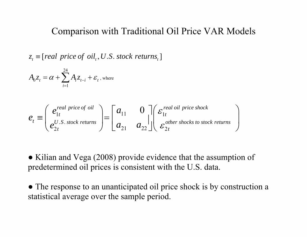
Comparison with Traditional Oil Price VAR Models
[ , . . ]t t tz real price of oil U S stock returns≡
24
01
t i t i ti
A z A zα ε−=
= + +∑ , where
111 1. .
21 222 2
0real price of oil real oil price shockt t
t U S stock returns other shocks to stock returnst t
aee
a aeεε
⎛ ⎞ ⎛ ⎞⎡ ⎤≡ =⎜ ⎟ ⎜ ⎟⎢ ⎥
⎣ ⎦⎝ ⎠ ⎝ ⎠
● Kilian and Vega (2008) provide evidence that the assumption of predetermined oil prices is consistent with the U.S. data. ● The response to an unanticipated oil price shock is by construction a statistical average over the sample period.
0 5 10 15-3
-2
-1
0
1
2
3Real oil price shock
Cum
ulat
ive
Rea
l Sto
ck R
etur
ns (P
erce
nt)
Months
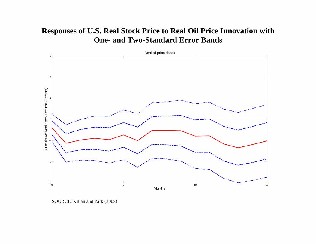
Responses of U.S. Real Stock Price to Real Oil Price Innovation with One- and Two-Standard Error Bands
SOURCE: Kilian and Park (2008)
7
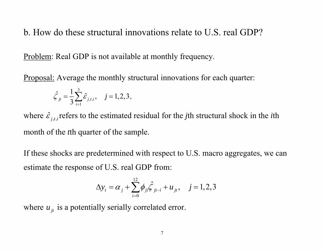
b. How do these structural innovations relate to U.S. real GDP? Problem: Real GDP is not available at monthly frequency.
Proposal: Average the monthly structural innovations for each quarter: 3
, ,1
1ˆ ˆ , 1,2,33jt j t i
i
jζ ε=
= =∑ ,
where , ,ˆ j t iε refers to the estimated residual for the jth structural shock in the ith
month of the tth quarter of the sample.
If these shocks are predetermined with respect to U.S. macro aggregates, we can
estimate the response of U.S. real GDP from:
12
0
ˆ , 1,2,3t j ji jt i jti
y u jα φ ζ −=
Δ = + + =∑
where jtu is a potentially serially correlated error.
0 2 4 6 8 10 12-10
-5
0
5
Rea
l GD
P
Crude Oil Supply Shock
0 2 4 6 8 10 12-10
-5
0
5
Rea
l GD
PAggregate Demand Shock
0 2 4 6 8 10 12-10
-5
0
5
Rea
l GD
P
Oil-Market Specific Demand Shock
Quarters
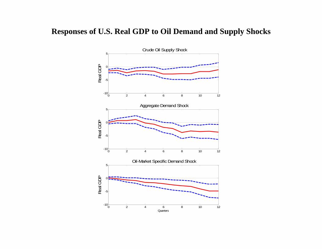
Responses of U.S. Real GDP to Oil Demand and Supply Shocks
1975 1980 1985 1990 1995 2000 2005
-100
-50
0
50
100
Real price of crude oilReal price of gasoline
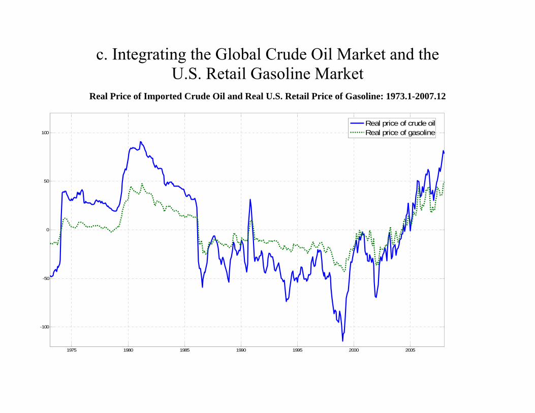
c. Integrating the Global Crude Oil Market and the U.S. Retail Gasoline Market
Real Price of Imported Crude Oil and Real U.S. Retail Price of Gasoline: 1973.1-2007.12
2
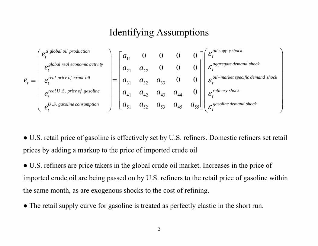
Identifying Assumptions
11
21 22
31 32 33
. .41 42 43 44
. . 51 52 53 45 55
0 0 0 00 0 0
0 00
global oil productiont
global real economic activitytreal price of crude oil
t treal U S price of gasolinetU S gasoline consumptiont
● U.S. retail price of gasoline is effectively set by U.S. refiners. Domestic refiners set retail
prices by adding a markup to the price of imported crude oil
● U.S. refiners are price takers in the global crude oil market. Increases in the price of
imported crude oil are being passed on by U.S. refiners to the retail price of gasoline within
the same month, as are exogenous shocks to the cost of refining.
● The retail supply curve for gasoline is treated as perfectly elastic in the short run.
0 5 10 15 20
-4
-2
0
2
4Refining shock
Rea
l pric
e of
oil
0 5 10 15 20-1.5
-1
-0.5
0
0.5
1
1.5Gas demand shock
Rea
l pric
e of
oil
Months0 5 10 15 20
-1.5
-1
-0.5
0
0.5
1
1.5Gas demand shock
Rea
l gas
pric
e
Months
0 5 10 15 20
-4
-2
0
2
4Refining shock
Rea
l gas
pric
e
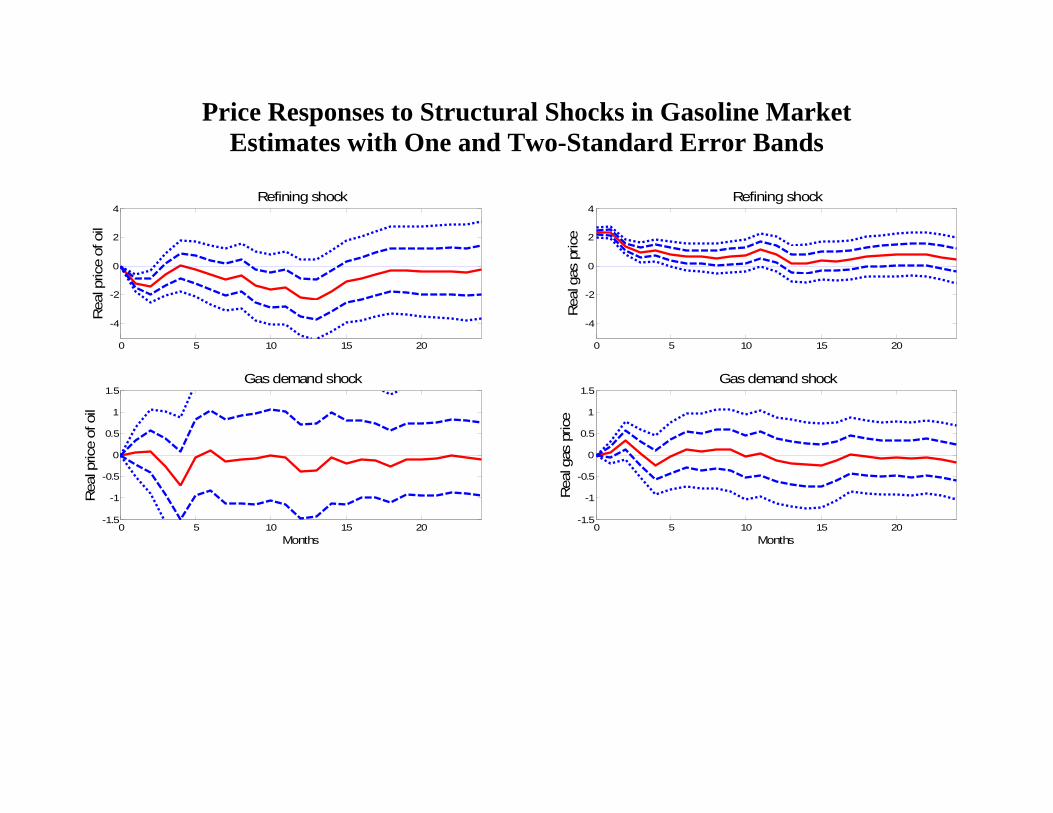
Price Responses to Structural Shocks in Gasoline Market Estimates with One and Two-Standard Error Bands
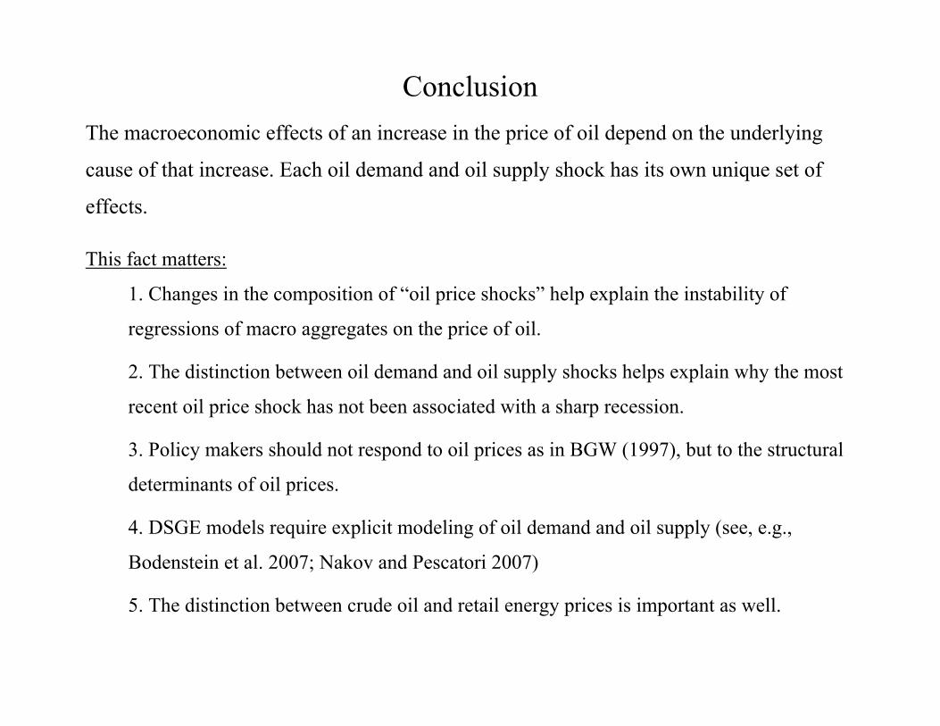
Conclusion The macroeconomic effects of an increase in the price of oil depend on the underlying
cause of that increase. Each oil demand and oil supply shock has its own unique set of
effects.
This fact matters:
1. Changes in the composition of “oil price shocks” help explain the instability of
regressions of macro aggregates on the price of oil.
2. The distinction between oil demand and oil supply shocks helps explain why the most
recent oil price shock has not been associated with a sharp recession.
3. Policy makers should not respond to oil prices as in BGW (1997), but to the structural
determinants of oil prices.
4. DSGE models require explicit modeling of oil demand and oil supply (see, e.g.,
Bodenstein et al. 2007; Nakov and Pescatori 2007)
5. The distinction between crude oil and retail energy prices is important as well.
Part 5:
Implications for DSGE Models of the
Transmission of Oil Demand and Supply Shocks
The Channels of Transmission in the Literature
A. Production (or cost) channels:
Direct Effects:
● The transmission of oil price shocks involves moving capital and labor inputs (unlike a technology shock). ● Direct effect is bounded by oil share in production and small (Backus and Crucini 2000). (U.S.: only ~3.5% in 1977, 2005) Indirect Effects:
Rotemberg and Woodford 1996: Large and time-varying markups
Atkeson and Kehoe 1999: Capital-energy complementarities
Finn 2000: Energy is essential to obtaining service flow from capital It is unclear whether these models can account for a large share of the business cycle or what their microeconomic support is.
B. Consumption/investment expenditure (or demand) channels:
An increase in energy prices slows economic growth primarily through its effects on consumer spending (Bernanke 2006).
Previous empirical studies: Lee and Ni (2002) provide survey evidence that oil shocks are viewed as demand rather than supply or cost shocks at industry level. Kilian and Park (2008) provide complementary evidence in favor of the demand channel based on industry-level stock returns. Edelstein and Kilian (2007a,b) quantify the energy share in consumption and investment expenditures and the importance of the demand channel. Problem: We need some amplifier since the energy share in expenditures is small. Some DSGE modeling by Hamilton (1988), Dhawan and Jeske (2007).
C. Monetary policy channel: Bernanke, Gertler, Watson (BPEA 1997):
● Fed creates recession by tightening monetary policy in response to fears that oil price shocks are inflationary. ● Without that policy reaction, the effects of oil price shocks on real output would be more benign. ● Recessions could have been avoided, had the Fed kept interest rates constant.
Problems: 1. It is not clear theoretically why the Fed should respond to oil price shocks (nor how large the effects of such a response would be).
2. It is not clear empirically that the Fed did respond to oil price shocks as presumed by BGW, or that the responses made a large difference.
3. The BGW estimates are weak, not robust, and inconsistent.
D. Real Wage Rigidities/Wage-Price Spirals: Bruno and Sachs (1985): In the presence of a downward-rigid real wage, unemployment may arise in response to an oil price shock. Problems: 1. Unions as the ultimate cause? (More plausible for Europe than the U.S.)
2. No direct evidence in support of real wage rigidities for either.
3. In the U.S. the aggregate real wage fell in response to oil price shocks. E. Oil and the Productivity Slowdown: Problems: 1. Labor productivity versus total factor productivity. 2. Timing? 3. Causality? 4. Empirical evidence mixed.
Demand Channels of Transmission (1): The Discretionary Income Effect
Higher energy prices are expected to reduce discretionary income, as consumers have less money to spend after paying their energy bills. The purchasing power gains and losses associated with energy price shocks are approximately the percent change in retail energy prices weighted by the time-varying share of energy expenditures in total expenditures. All else equal, this discretionary income effect will be the larger, the less elastic the demand for energy, but even with perfectly inelastic energy demand the magnitude of the effect of a unit change in energy prices is bounded by the energy share in consumption.
Caveats on the Discretionary Income Effect
1. Implicit is the assertion:
(1) Higher energy prices are primarily driven by higher prices for imported energy goods.
(2) Discretionary income lost from higher prices of imported energy goods is transferred abroad and is not recycled in the form of higher U.S. exports (or returns on foreign asset holdings).
(3) High share of energy in expenditures (U.S.: only ~6.5% in 1970, 2005)
2. In the case of a purely domestic energy price shock (such as a shock to U.S. refining capacity), it is even less obvious that there is an effect on aggregate discretionary income.
The transfer of income to the refiner may be partially returned to consumers in the form of higher wages or higher stock returns on domestic energy companies. Even if the transfer is not returned, higher energy prices simply constitute an income transfer from one consumer to another that cancels in the aggregate.
Demand Channels of Transmission (2): The Uncertainty Effect
Changing energy prices may create uncertainty about the future path of the price of energy, causing consumers to postpone irreversible purchases of consumer durables (see Bernanke 1983, Pindyck 1991). Unlike the discretionary income effect, this uncertainty effect is limited to consumer durables.
Demand Channels of Transmission (3): The Precautionary Savings Effect
Even when purchase decisions are reversible, consumption may fall in response to energy price shocks, as consumers increase their precautionary savings. This response may arise if consumers smooth their consumption because they perceive a greater likelihood of future unemployment and hence future income losses. It may also reflect greater uncertainty about the prospects of remaining gainfully employed (in which case any change in energy prices would lower consumption).
Demand Channels of Transmission (4): The Operating Cost Effect
Consumption of durables whose operation requires energy will decline, as households delay or forego purchases of energy-using durables. As the dollar value of such purchases may be large relative to the value of the energy they use, even relatively small changes in energy prices (and hence in purchasing power) can have large effects on expenditures. This operating cost effect is more limited in scope than the uncertainty effect in that it only affects specific consumer durables. It should be most pronounced for motor vehicles.
Demand Channels of Transmission (5): The Reallocation Effect
Shifts in expenditure patterns driven by the uncertainty effect and operating cost effect amount to allocative disturbances that are likely to cause sectoral shifts throughout the economy:
1. Reduced expenditures on energy-intensive durables such as automobiles may cause the reallocation of capital and labor away from the automobile sector (Hamilton 1988).
A similar reallocation may occur within the same sector, as consumers switch toward more energy-efficient durables (Bresnahan and Ramey 1993).
2. In the presence of frictions in capital and labor markets, these reallocations will cause resources to be unemployed, thus causing further cutbacks in consumption and amplifying the effect of energy price shocks on the real economy.
This reallocation effect could be much larger than the direct effects listed earlier.
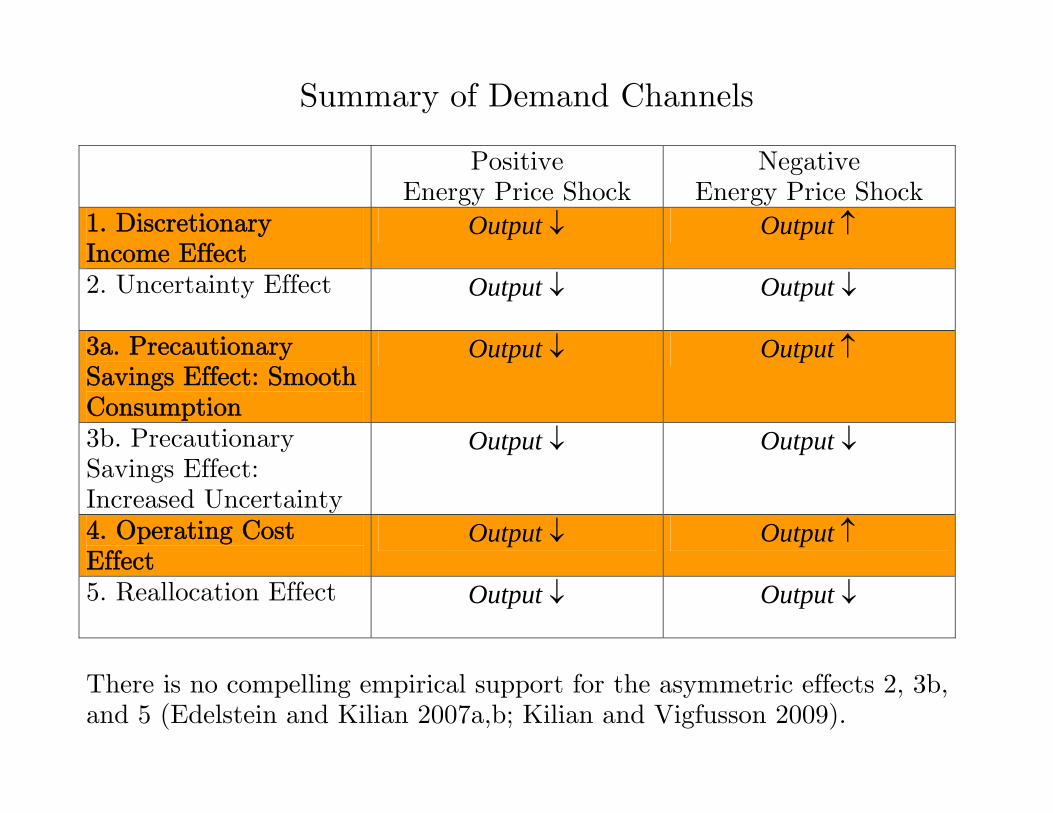
There is no compelling empirical support for the asymmetric effects 2, 3b, and 5 (Edelstein and Kilian 2007a,b; Kilian and Vigfusson 2009).
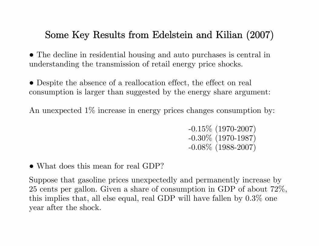
Some Key Results from Edelstein and Kilian (2007) ● The decline in residential housing and auto purchases is central in understanding the transmission of retail energy price shocks. ● Despite the absence of a reallocation effect, the effect on real consumption is larger than suggested by the energy share argument: An unexpected 1% increase in energy prices changes consumption by: -0.15% (1970-2007) -0.30% (1970-1987) -0.08% (1988-2007) ● What does this mean for real GDP?
Suppose that gasoline prices unexpectedly and permanently increase by 25 cents per gallon. Given a share of consumption in GDP of about 72%, this implies that, all else equal, real GDP will have fallen by 0.3% one year after the shock.
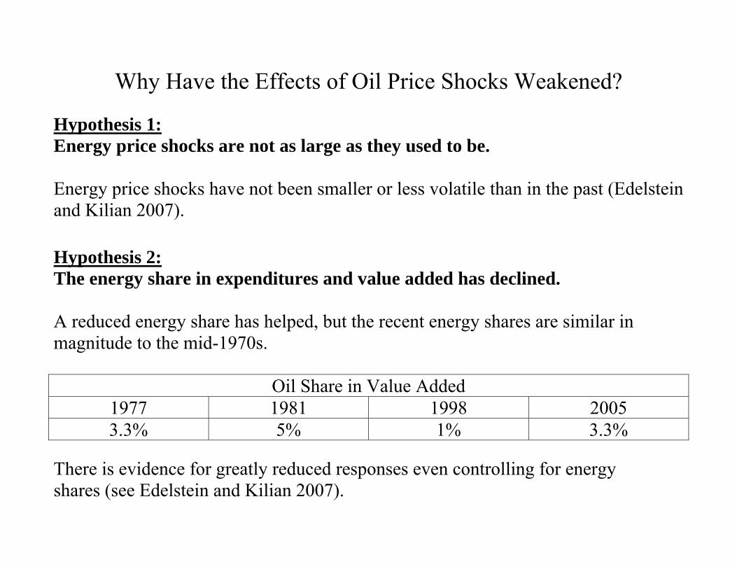
Why Have the Effects of Oil Price Shocks Weakened? Hypothesis 1: Energy price shocks are not as large as they used to be. Energy price shocks have not been smaller or less volatile than in the past (Edelstein and Kilian 2007).
Hypothesis 2: The energy share in expenditures and value added has declined. A reduced energy share has helped, but the recent energy shares are similar in magnitude to the mid-1970s.
Oil Share in Value Added 1977 1981 1998 2005 3.3% 5% 1% 3.3%
There is evidence for greatly reduced responses even controlling for energy shares (see Edelstein and Kilian 2007).
Hypothesis 3: The product mix of the U.S. auto industry has changed.
In the 1970s, the U.S. did not produce small, energy efficient cars, so every auto
sale lost to imports caused a reduction in employment. Today, domestic and foreign
auto producers are more similar (Edelstein and Kilian 2007).
0 2 4 6 8 10 12 14 16 18
-7
-6
-5
-4
-3
-2
-1
0
1
2
3
Perc
ent
New Domestic Autos: 1970.2-1987.12
0 2 4 6 8 10 12 14 16 18
-7
-6
-5
-4
-3
-2
-1
0
1
2
3
New Domestic Autos: 1988.1-2006.7
Months
Perc
ent
0 2 4 6 8 10 12 14 16 18
-7
-6
-5
-4
-3
-2
-1
0
1
2
3
New Foreign Autos: 1970.2-1987.12
0 2 4 6 8 10 12 14 16 18
-7
-6
-5
-4
-3
-2
-1
0
1
2
3
Months
New Foreign Autos: 1988.1-2006.7
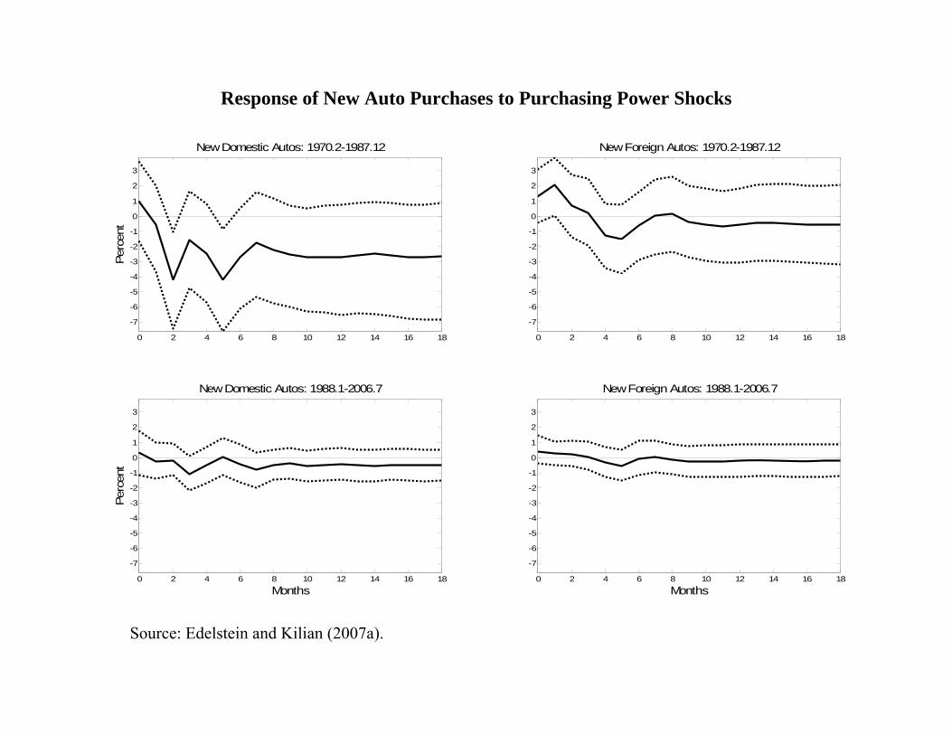
Response of New Auto Purchases to Purchasing Power Shocks
Source: Edelstein and Kilian (2007a).
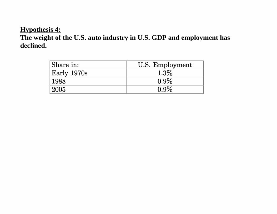
Hypothesis 4: The weight of the U.S. auto industry in U.S. GDP and employment has declined.
Share in: U.S. Employment Early 1970s 1.3% 1988 0.9% 2005 0.9%
Hypothesis 5: The composition of oil price shocks has changed.
● The effect of an increase in the price of oil depends on the underlying cause of
that increase.
● Each oil demand and oil supply shock has its own unique set of dynamic
effects. The net effect depends on the composition of oil demand and supply
shocks.
● The distinction between oil demand and oil supply shocks helps explain why
the most recent oil price shock has not been associated with a sharp recession.
1979 1980 1981 1982 1983 1984 1985 1986
-10
-5
0
5
10
15
Dem
eane
d U
.S. C
PI In
flatio
n
1979-1986
2002 2003 2004 2005 2006 2007 2008
-10
-5
0
5
10
15
Dem
eane
d U
.S. C
PI In
flatio
n
2002-2008
2002 2003 2004 2005 2006 2007 2008
-10
-5
0
5
10
15
Dem
eane
d U
.S. R
eal G
DP
Gro
wth
2002-2008
1979 1980 1981 1982 1983 1984 1985 1986
-10
-5
0
5
10
15
Dem
eane
d U
.S. R
eal G
DP
Gro
wth
1979-1986
Total Cumulative EffectActual
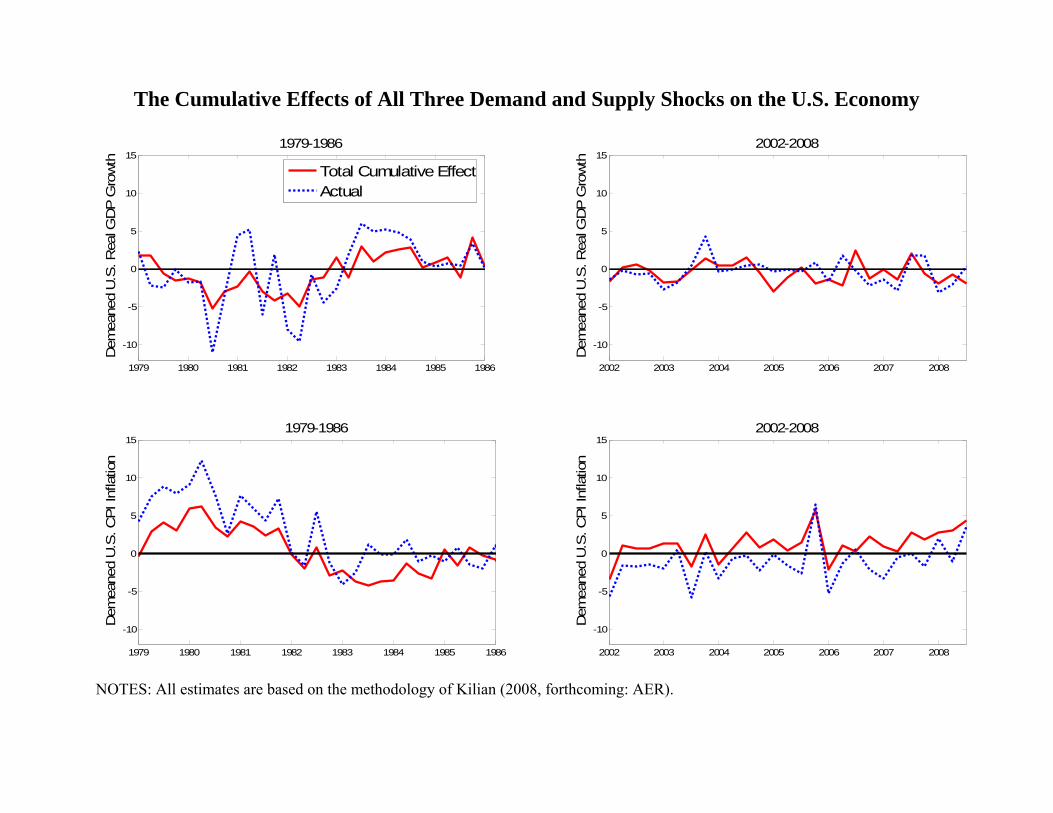
The Cumulative Effects of All Three Demand and Supply Shocks on the U.S. Economy
NOTES: All estimates are based on the methodology of Kilian (2008, forthcoming: AER).
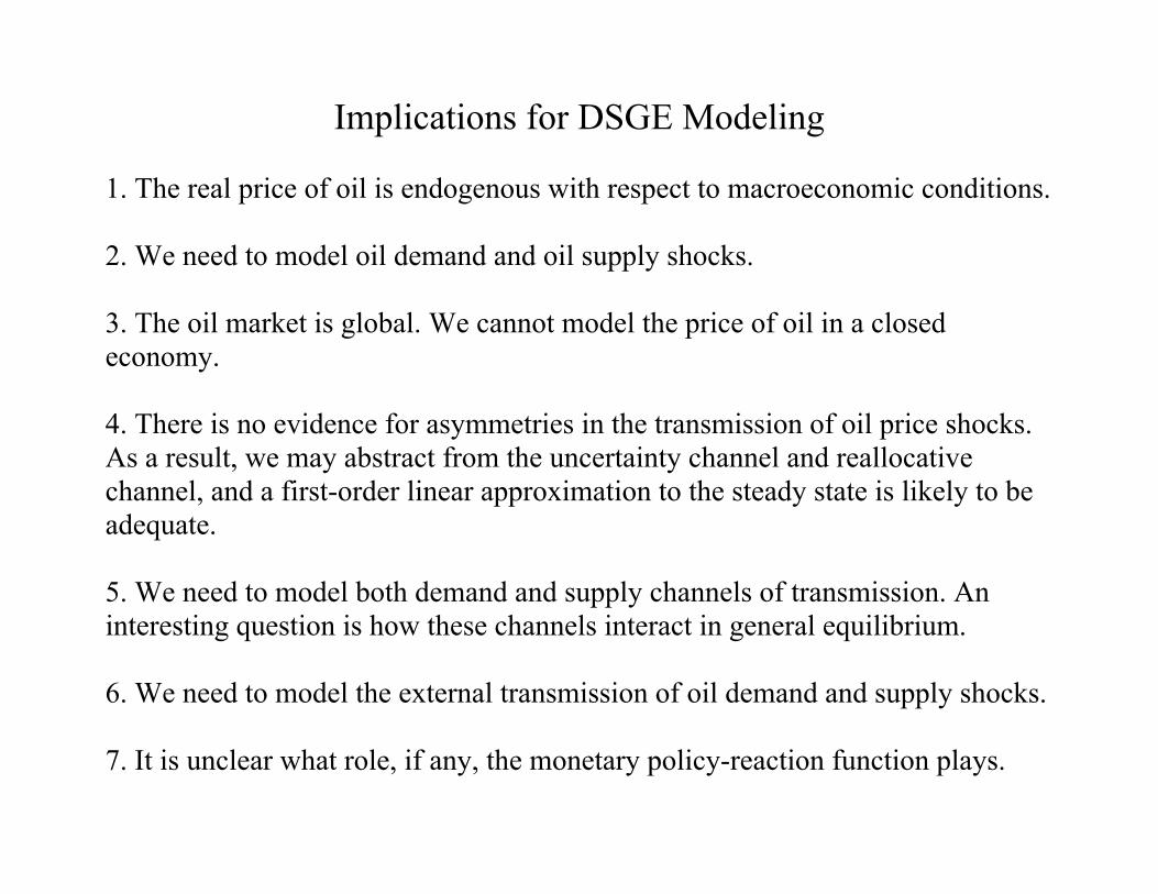
Implications for DSGE Modeling 1. The real price of oil is endogenous with respect to macroeconomic conditions. 2. We need to model oil demand and oil supply shocks. 3. The oil market is global. We cannot model the price of oil in a closed economy. 4. There is no evidence for asymmetries in the transmission of oil price shocks. As a result, we may abstract from the uncertainty channel and reallocative channel, and a first-order linear approximation to the steady state is likely to be adequate. 5. We need to model both demand and supply channels of transmission. An interesting question is how these channels interact in general equilibrium. 6. We need to model the external transmission of oil demand and supply shocks. 7. It is unclear what role, if any, the monetary policy-reaction function plays.
5
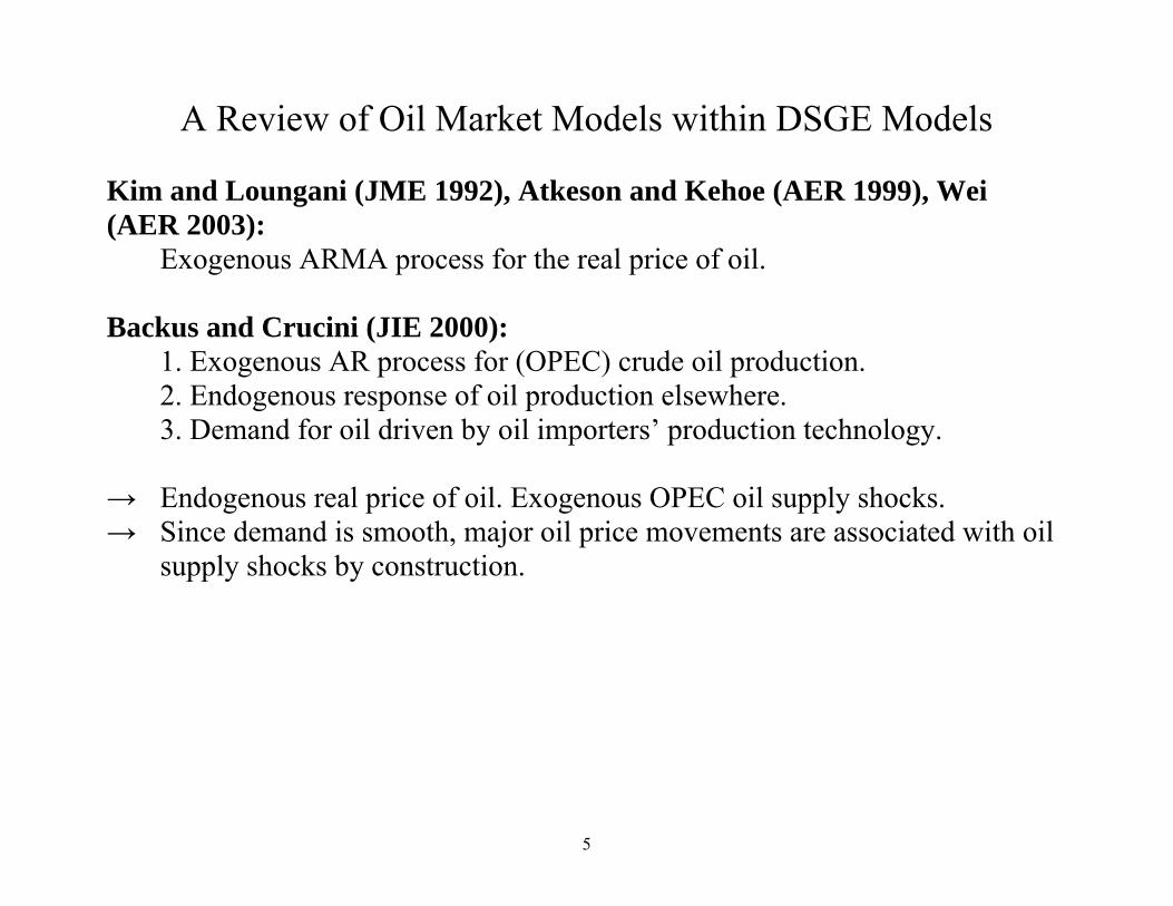
A Review of Oil Market Models within DSGE Models Kim and Loungani (JME 1992), Atkeson and Kehoe (AER 1999), Wei (AER 2003): Exogenous ARMA process for the real price of oil. Backus and Crucini (JIE 2000): 1. Exogenous AR process for (OPEC) crude oil production. 2. Endogenous response of oil production elsewhere. 3. Demand for oil driven by oil importers’ production technology. → Endogenous real price of oil. Exogenous OPEC oil supply shocks. → Since demand is smooth, major oil price movements are associated with oil supply shocks by construction.
Bodenstein, Erceg and Guerrieri (2007): 1. Oil supply shocks as exogenous shocks to crude oil production as in BC 2000.
2. Oil-market specific demand modeled as a “foreign” preference shock.
Narrow interpretation: Exogenous oil taste shift in China. Loose interpretation: Reduced form for expectation shifts.
Nakov and Pescatori (2008, forthcoming: EJ): 1. OPEC oil supply is endogenous.
3. Structural disturbances to oil importers’ productivity, technology in the oil sector, and the capacity of the competitive fringe of oil producers.
4. No oil-market specific demand.
Balke, Brown, and Yücel (2008): 1. Oil supply is endogenous.
2. Reserves are required to produce oil. There are technology shocks to the production of reserves and to the production of oil. Oil producers are oil price takers.
3. Oil-demand shocks mainly arise from domestic and foreign productivity gains plus an “oil wedge” (= energy efficiency) shock.
4. No oil-specific demand shocks.
The Next Generation of Models
1. Calibrated models are of limited usefulness for policy analysis in that they allow for a wide range of responses to oil demand and oil supply shocks. We need to estimate these models to pin down the relevant magnitudes. This requires more attention to details of the model specification, for estimates are only as credible as the underlying model. 2. Recent DSGE models have focused on selected demand and supply shocks in isolation. We need a model that includes all three types of shocks at the same time. At a minimum, we need oil-specific demand shocks, aggregate demand shocks and oil supply shocks. 3. A case can be made that we need to distinguish further between different sources of aggregate demand shocks (e.g., foreign productivity versus domestic and/or foreign monetary expansion as in the 1970s). This distinction also matters in that monetary-policy driven demand shocks have purely transitory effects, whereas foreign productivity shocks might have permanent effects on the real price of oil.
4. We need a sufficiently long estimation period to ensure the identification of these oil demand and supply shocks. 5. It is important that we distinguish between retail energy prices (such as the price of gasoline) and the price of crude oil. We need to model both the crude oil market and the refinery market, since crude oil is not consumed directly. 6. We need to allow for both supply/cost/production channels of transmission and demand/consumption channels. Ultimately, models will have to flesh out the role of the automobile sector and of the residential housing sector. A multi-sector model may be useful in that respect. 7. We need to allow for the evolution of the energy share on the cost and expenditure side. 8. Technology shocks are not a good proxy for shocks to the aggregate demand for industrial commodities.