22
A Subexponential Bound for Linear Programming
�y
Ji
�
r
�
i Matou
�
sek
z
Department of Applied Mathematics
Charles University, Malostransk�e n�am. 25
118 00 Praha 1, Czechoslovakia
e-mail: [email protected]
Micha Sharir
School of Mathematical Sciences
Tel Aviv University, Tel Aviv 69978, Israel
e-mail: [email protected]
and
Courant Institute of Mathematical Sciences
New York University, New York, NY 10012, USA
Emo Welzl
Institut f�ur Informatik, Freie Universit�at Berlin
Takustra�e 9, 14195 Berlin, Germany
e-mail: [email protected]
Abstract
We present a simple randomized algorithm which solves linear programs
with n constraints and d variables in expected
minfO(d
2
2
d
n); e
2
p
d ln(n=
p
d )+O(
p
d+lnn)
g
time in the unit cost model (where we count the number of arithmetic oper-
ations on the numbers in the input); to be precise, the algorithm computes
the lexicographically smallest nonnegative point satisfying n given linear in-
equalities in d variables. The expectation is over the internal randomizations
�
Work by the �rst author has been supported by a Humboldt Research Fellowship. Work by
the second and third authors has been supported by the German-Israeli Foundation for Scienti�c
Research and Development (G.I.F.). Work by the second author has been supported by O�ce of
Naval Research Grant N00014-90-J-1284, by National Science Foundation Grants CCR-89-01484
and CCR-90-22103, and by grants from the U.S.-Israeli Binational Science Foundation, and the
Fund for Basic Research administered by the Israeli Academy of Sciences.
y
A preliminary version appeared in Proc. 8th Annual ACM Symposium on Computational
Geometry, 1992, pages 1{8.
z
Work has been carried out while author was visiting the Institute for Computer Science, Berlin
Free University
1

performed by the algorithm, and holds for any input. In conjunction with
Clarkson's linear programming algorithm, this gives an expected bound of
O(d
2
n+ e
O(
p
d lnd)
) :
The algorithm is presented in an abstract framework, which facilitates
its application to several other related problems like computing the smallest
enclosing ball (smallest volume enclosing ellipsoid) of n points in d-space,
computing the distance of two n-vertex (or n-facet) polytopes in d-space, and
others. The subexponential running time can also be established for some of
these problems (this relies on some recent results due to G�artner).
KEYWORDS: computational geometry, combinatorial optimization, linear pro-
gramming, smallest enclosing ball, smallest enclosing ellipsoid, randomized incre-
mental algorithms.
1 Introduction
Linear programming is one of the basic problems in combinatorial optimization, and
as such has received considerable attention in the last four decades. Many algorithms
have been proposed for its solution, starting with the simplex algorithm and its rel-
atives [Dan], proceeding through the polynomial-time solutions of Khachiyan [Kha]
and Karmarkar [Kar], and continuing with several more recent techniques (reviewed
below). While some of the proposed algorithms have proven out to be extremely
e�cient in practice, analysis of their running time has not been fully satisfactory so
far. For example, the simplex algorithm was shown to be exponential in the worst
case [KlM]. The algorithms of Khachiyan and of Karmarkar have polynomial bit-
complexity, but the number of arithmetic operations they perform depends on the
size of the coe�cients de�ning the input and it cannot be bounded solely in terms
of n (the number of constraints) and d (the number of variables). In this paper
we assume a di�erent model of computation, namely the real RAM, widely used in
computational geometry. Here the input may contain arbitrary real numbers, and
each arithmetic operation with real numbers is charged unit cost. To distinguish
complexity bounds in this model from bounds in the bit-complexity model, we call
them combinatorial.
Until recently, the best known combinatorial bounds were exponential in either
n or d; a subexponential (randomized) bound is given in a very recent paper of Kalai
[Kal] and also in this paper. One of the major open problems in the area is to �nd
a strongly polynomial algorithm (i.e. of combinatorial polynomial complexity) for
linear programming.
In this paper we describe a simple randomized algorithm which solves linear
programs with n inequalities and d variables with expected
O(minfd
2
2
d
n; e
2
p
d ln(n=
p
d )+O(
p
d+lnn)
g)
2

arithmetic operations. In conjunction with Clarkson's linear programming algorithm
[Cla3], this gives an expected bound of
O(d
2
n+ e
O(
p
d lnd)
) :
The expectation of the running time is with respect to the internal randomizations
performed by the algorithm, and holds for any input. This complexity matches that
of a recent algorithm due to Kalai [Kal]. (Except for the constant in the exponent,
the only signi�cant di�erence is that Kalai has a version of his algorithm which
runs in e
O(
p
d)
as long as n is linear in d. We can guarantee this bound only for
n = O(
p
d).) Chronologically speaking, our algorithm was published �rst in [ShW],
but with a weaker analysis of its running time; Kalai's analysis with a subexponential
bound came next, and immediately afterwards we realized that our algorithm also
has subexponential running time.
The algorithm is presented in an abstract framework which facilitates the ap-
plication of the algorithm to a large class of problems, including the computation
of smallest enclosing balls (or ellipsoids) of �nite point sets in d-space, comput-
ing largest balls (ellipsoids) in convex polytopes in d-space, computing the distance
between polytopes in d-space, etc. (however, we can guarantee a subexponential
running time for only some of these problems; see below for details).
To compare the complexity of our algorithm with other recent techniques, here
is a brief survey of some relevant recent literature. Megiddo [Meg2] has given the
�rst deterministic algorithm whose running time is of the form O(C
d
n), and is
thus linear in n for any �xed d. However the factor C
d
in his algorithm is 2
2
d
; an
improvement to C
d
= 3
d
2
can be found in [Dye1] and [Cla1]. Recently, a number
of randomized algorithms have been presented for the problem, see [DyF], [Cla3],
[Sei1], with a better dependence on d, where the best expected running time is
given by Clarkson [Cla3]: O(d
2
n + d
d=2+O(1)
log n). Nevertheless, the dependence
on d is still exponential. The more recent algorithm of Seidel [Sei1] has worse
expected complexity of O(d!n), but is an extremely simple randomized incremental
algorithm. In [Wel] this algorithm was enhanced with a \move-to-front" heuristic,
which in practice has drastically improved the performance of the algorithm, but was
(and still is) very di�cult to analyze. Our algorithm is another variant, in-between
the techniques of [Sei1] and [Wel]. (It is interesting, that there are examples of
linear programs (with few constraints), where adding the move-to-front heuristic to
our new algorithm gives a signi�cantly worse performance [Mat1].) Our algorithm
also seems to behave well in practice, and its analysis, as given here, also provides a
considerably improved worst-case upper bound on its expected complexity. Recently,
derandomization techniques have been applied to Clarkson's algorithm to obtain
deterministic O(C
d
n) time LP algorithms with C
d
of the order 2
O(d logd)
[ChM].
The abstract framework we present considers the set H of n constraints, and a
function w which maps every subset of H to its optimal solution, where w satis�es
a few simple conditions; as it turns out, this is all which is needed to prove the
correctness of the algorithm, and to analyze its expected running time in terms of
two primitive operations | `violation tests' and `basis computations'. It turns out
3

that these primitive operations can easily be implemented in polynomial time for
linear programming, but that is by no means clear for other instances of problems
in the framework. For example in the case of computing the smallest enclosing ball,
a basis computation amounts to computing the smallest ball enclosing d+ 2 points
in d-space. Only recently, G�artner [G�ar2] was able to show that this can be done
with expected e
O(
p
d)
arithmetic operations.
Clarkson's algorithm [Cla3] can also be shown to work in this framework, while
the algorithm of Seidel [Sei1] (and the generalization to other applications in [Wel])
needs to make a more explicit use of the geometry of the problems. A di�erent
framework has been recently developed by Dyer [Dye2], which yields deterministic
algorithms linear in n (with larger constants in d).
The paper is organized as follows. In the next section we introduce some nota-
tions and review basic observations on linear programming that are required for the
presentation and analysis of our algorithm in Section 3. The analysis culminates in
a recurrence relationship, whose solution is a nontrivial and interesting task in itself;
Section 4 is devoted to that solution. Finally, in Section 5 we describe the abstract
framework, and mention a few examples.
2 Notation and Basics
In the following we will prepare the notation required for our presentation. We
model the case of linear programming where the objective function is de�ned by the
vertical vector c = (�1; 0; 0 : : : ; 0), and the problem is to maximize c � x over an
intersection of given n halfspaces.
We let `<' be the lexicographical ordering on R
d
, (i.e. x < x
0
, if x
1
< x
0
1
, or
x
1
= x
0
1
and x
2
< x
0
2
, or so on). This ordering is extended to R
d
[ f+1;�1g (
+1 and �1 being special symbols) by the convention that �1 < x < +1 for all
x 2 R
d
.
Let H be a set of closed halfspaces in d-space (which we call also constraints in
d-space). By v
H
we denote the lexicographically smallest point in the feasible region
F
H
:=
T
h2H
h; v
H
is called the value of H. (It seems more standard to look for the
backwards lexicographically smallest point, i.e., the case when c = (0; 0; : : : ; 0;�1);
the reader accustomed to this may prefer to think `backwards' instead.) If F
H
is
empty, then we let v
H
= +1. If F
H
is nonempty, but contains no minimum, then
we let v
H
= �1.
Intuitively, we can view +1 as a point which lies in all halfspaces and which
dominates all points. �1 may be seen as a point in minus in�nity, or simply as a
symbol for `unde�ned'.
A basis B is a set of constraints with �1 < v
B
, and v
B
0
< v
B
for all proper
subsets B
0
of B. If �1 < v
H
, a basis of H is a minimal subset B ofH with v
B
= v
H
.
Constraint h is violated by H, if v
H
< v
H[fhg
; if �1 < v
H
, then this is equivalent
to v
H
62 h. Constraint h is extreme in H, if v
H�fhg
< v
H
. Note that h is extreme in
H if and only if h 2 H and h is violated by H � fhg.
4

The following properties are either trivial (like (i) and (ii)), or standard in linear
programming theory (like (iii)). We cite them explicitly here, because they consti-
tute all that is needed for the correctness and time analysis of the algorithms to be
described.
Lemma 1 Let G and H be sets of constraints in d-space, G � H, and let h be a
constraint in d-space.
(i) v
G
� v
H
.
(ii) If �1 < v
G
= v
H
, then h is violated by G if and only if h is violated by H.
(iii) If v
H
< +1, then any basis B � H has exactly d constraints, and any F � H
has at most d extreme constraints.
3 The Algorithm
Let H
+
be the set of constraints x
i
� 0, for 1 � i � d. Given a set H of constraints,
the following algorithm will compute a basis of H [H
+
; such a basis always exists,
because �1 < (0; 0; : : : ; 0) � v
H[H
+
. (The algorithm works for any initial basis B
0
instead of H
+
; in particular, we could take any basis B
0
� H, if available, or we can
take a set of constraints x
i
� �!, 1 � i � d, for a symbolic value �! representing
an arbitrarily small number.) We will always assume that v
H[H
+
< +1 for the
constraint sets we consider. It is well-known that this condition can be obtained at
the cost of an extra dimension and an extra constraint. However, note that we have
not made any general position assumptions; so, e.g., we do not require that bases
are unique.
Given a set H of n constraints, we might �rst consider the following trivial
approach. Remove a random constraint h, and compute a basis B for H � fhg
recursively. If h is not violated by B (or equivalently, if h is not violated byH�fhg),
then B is a basis for H and we are done. If h is violated, then we try again by
removing a (hopefully di�erent) random constraint. Note that the probability that
h is violated by H �fhg is at most
d
n
since there are at most d extreme constraints
in H.
So much for the basic idea, which we can already �nd in Seidel's LP algorithm
[Sei1]; however, in order to guarantee e�ciency, we need some additional ingredients.
First, the procedure SUBEX lp actually solving the problem has two parameters: the
set H of constraints, and a basis C � H; in general, C is not a basis of H, and we
call it a candidate basis. It can be viewed as some auxiliary information we get for
the computation of the solution. Note that C has no in uence on the output of the
procedure (but it in uences its e�ciency).
The problem of computing a basis of H [H
+
can now be solved by:
function procedure subex lp(H); /* H : set of n constraints in d-space;
B := SUBEX lp(H [H
+
; H
+
); /* returns a basis of H [H
+
.
return B;
5

The following pseudocode for SUBEX lp uses two primitive operations: The �rst is
a test `h is violated by B', for a constraint h and a basis B (violation test); this
operation can be implemented in time O(d), if we keep v
B
with the basis B. Second,
SUBEX lp assumes the availability of an operation, `basis(B;h)', which computes
a basis of B [ fhg for a d-element basis B and a constraint h (basis computation).
This step corresponds to a pivot step, and with an appropriate representation of B,
it can be performed with O(d
2
) arithmetic operations. Note that if �1 < v
B
, then
�1 < v
B[fhg
, and so �1 < v
H
for all constraint sets H considered in an execution.
function procedure SUBEX lp(H;C); /* H : set of n constraints in d-space;
if H = C then /* C � H : a basis;
return C /* returns a basis of H .
else
choose a random h 2 H � C;
B := SUBEX lp(H � fhg; C);
if h is violated by B then /* , v
B
62 h
return SUBEX lp(H; basis(B; h))
else
return B;
A simple inductive argument shows that the procedure returns the required
answer. This happens after a �nite number of steps, since the �rst recursive call
decreases the number of constraints, while the second call increases the value of the
candidate basis (and there are only �nitely many di�erent bases).
For the analysis of the expected behavior of the algorithm, let us take a closer
look at the probability that the algorithm makes the second recursive call with
candidate basis `basis(B;h)'. As noted above, this happens exactly when h is
extreme in h. Since we now choose h from H �C (and C always has d elements), it
follows that the probability for h being extreme is at most
d
n�d
. Moreover, if d � k
extreme constraints in H are already in C, then the bound improves to
k
n�d
; in fact,
there are never more `bad' choices than there are choices at all, and so the bound
can be lowered to
minfn�d;kg
n�d
. We want to show that the numerator decreases rapidly
as we go down the recursion, and this will entail the subexponential time bound.
The key notion in our analysis will be that of hidden dimension. For given
G � H and a basis C � G, the hidden dimension of the pair (G;C) measures how
\close" is C to the solution (basis) of G. The hidden dimension of (G;C) is d minus
the number of constraints h 2 C which must be contained in any basis B � G with
value greater than or equal to the value of C.
Lemma 2 The hidden dimension of (G;C) is d� jfh 2 G; v
G�fhg
< v
C
gj.
Proof. We need to show that a constraint h 2 G satis�es v
G�fhg
< v
C
i� h
appears in all bases B � G with v
B
� v
C
. If v
G�fhg
< v
C
and B � G is a basis
with v
B
� v
C
, and h is not in B, then B � G � fhg, so v
B
� v
G�fhg
< v
C
, a
contradiction. Conversely, if v
G�fhg
� v
C
then let B be a basis for G � fhg. We
6

have v
B
= v
G�fhg
� v
C
and h is not in B. This completes the proof of the lemma.
Let us remark that the hidden dimension of (G;C) depends on C only via the
value of C. An intuitive interpretation is that all the \local optima" de�ned by
constraints of G lying above the \level" v
C
are contained in a k- at de�ned by some
d � k bounding hyperplanes of constraints of C, k being the hidden dimension.
Hidden dimension zero implies that C is a basis of G.
We enumerate the constraints in H in such a way that
v
H�fh
1
g
� v
H�fh
2
g
� � � � � v
H�fh
d�k
g
< v
C
� v
H�fh
d�k+1
g
� � � � � v
H�fh
n
g
:
The ordering is not unique, but the parameter k emerging from this ordering is
unique and, by de�nition, it equals the hidden dimension of (H;C).
Note that for h 2 H�C, v
C
� v
H�fhg
, and so h
1
; h
2
; : : : ; h
d�k
are in C. Hence the
only choices for h which possibly entail a second call are h
d�k+1
; : : : ; h
d
(for i > d,
v
H�fh
i
g
= v
H
). Suppose that, indeed, a constraint h
d�k+i
, 1 � i � k, is chosen,
and the �rst call (with candidate basis C) returns with basis B, v
B
= v
H�fh
d�k+i
g
.
Then we compute C
0
= basis(B;h
d�k+i
). Since v
H�fh
d�k+i
g
= v
B
< v
C
0
, the hidden
dimension of the pair (H;C
0
) for the second call is at most k � i.
The hidden dimension is monotone, i.e., if C � G � H, then the hidden dimen-
sion of (G;C) does not exceed the hidden dimension of (H;C). This holds, because
the constraints h
1
; h
2
; : : : ; h
d�k
are in C (and so in G), and v
G�fh
i
g
� v
H�fh
i
g
because
G � H.
We denote by t
k
(n) and b
k
(n) the maximum expected number of violation tests
and basis computations, respectively, entailed by a call SUBEX lp(H;C) with n con-
straints and hidden dimension � k. The discussion above yields the following re-
currence relationships: t
k
(d) = 0 for 0 � k � d,
t
k
(n) � t
k
(n� 1) + 1 +
1
n� d
minfn�d;kg
X
i=1
t
k�i
(n) for n > d ;
and b
k
(d) = 0 for 0 � k � d,
b
k
(n) � b
k
(n� 1) +
1
n� d
minfn�d;kg
X
i=1
(1 + b
k�i
(n)) for n > d: (3.1)
Simple proofs by induction show that b
k
(n) � 2
k
(n � d) and t
k
(n) � 2
k
(n � d). It
turns out that for n not much larger than d, this is a gross overestimate, and in the
next section we will show that
b
d
(n + d) � e
2
p
d ln(n=
p
d )+O(
p
d+lnn)
:
We have also t
k
(n) � (n � d)(1 + b
k
(n)); indeed, every constraint is tested at
most once for violation by B, for each basis B ever appearing in the computation;
we have tha factor (n � d) since we do not test the elements in B for violation by
B, and we add 1 to b
k
(n) to account for the initial basis H
+
.
7

Recall that we account O(d) arithmetic operations for a violation test, and O(d
2
)
arithmetic operations for a basis computation. Note also that for the computation of
v
H[H
+
, we have to add the d nonnegativity constraints before we initiate SUBEX lp.
Anticipating the solution of the recurrences, given in the next section, we thus
conclude:
Theorem 3 Let H be a set of n constraints in d-space. The lexicographically small-
est nonnegative point v
H[H
+
in the intersection of the halfspaces in H can be com-
puted by a randomized algorithm with an expected number of
O(nd + d
2
) b
d
(n+ d) = e
2
p
d ln(n=
p
d )+O(
p
d+lnn)
arithmetic operations.
Clarkson [Cla3] shows that a linear program with n constraints in d-space can be
solved with expected
O(d
2
n+ d
4
p
n log n+ T
d
(9d
2
)d
2
log n) (3.2)
arithmetic operations, where T
d
(9d
2
) stands for the complexity of solving a linear
program with 9d
2
constraints in d-space. We replace T
d
(9d
2
) by our bound, and
observe that, after this replacement, the middle term in (3.2) is always dominated
by the two other terms; moreover, we can even omit the `log n' factor in the last
term in (3.3) without changing the asymptotics of the whole expression. Thus, we
obtain:
Corollary 4 The lexicographically smallest nonnegative point v
H[H
+
in the inter-
section of the n halfspaces H in d-space can be computed by a randomized algorithm
with an expected number of
O(d
2
n+ e
O(
p
d logd)
) (3.3)
arithmetic operations.
4 Solving the Recurrence
In this section we prove the promised bounds for b
k
(n). We �rst put
^
b
k
(n) =
1 + b
k
(n + d), and we let f(k; n) be the function which satis�es the recurrence for
^
b
k
(n) with equality (thus majorizing
^
b
k
(n)).
Thus f(k; n) is the solution to the recurrence
f(k; 0) = f(0; n) = 1 for k; n � 0,
and
f(k; n) = f(k; n � 1) +
1
n
min(n;k)
X
j=1
f(k � j; n) for k; n � 1. (4.1)
We prove the following upper bound:
8
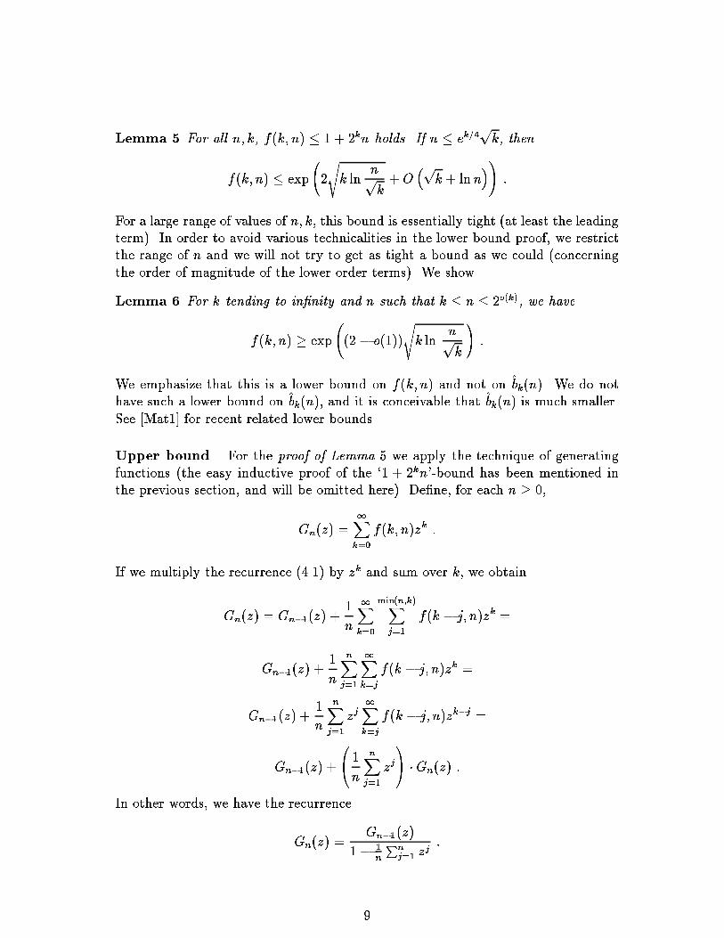
Lemma 5 For all n; k, f(k; n) � 1 + 2
k
n holds. If n � e
k=4
p
k, then
f(k; n) � exp
2
s
k ln
n
p
k
+O
�
p
k + ln n
�
!
:
For a large range of values of n; k, this bound is essentially tight (at least the leading
term). In order to avoid various technicalities in the lower bound proof, we restrict
the range of n and we will not try to get as tight a bound as we could (concerning
the order of magnitude of the lower order terms). We show
Lemma 6 For k tending to in�nity and n such that k � n � 2
o(k)
, we have
f(k; n) � exp
(2 � o(1))
s
k ln
n
p
k
!
:
We emphasize that this is a lower bound on f(k; n) and not on
^
b
k
(n). We do not
have such a lower bound on
^
b
k
(n), and it is conceivable that
^
b
k
(n) is much smaller.
See [Mat1] for recent related lower bounds.
Upper bound. For the proof of Lemma 5 we apply the technique of generating
functions (the easy inductive proof of the `1 + 2
k
n'-bound has been mentioned in
the previous section, and will be omitted here). De�ne, for each n � 0,
G
n
(z) =
1
X
k=0
f(k; n)z
k
:
If we multiply the recurrence (4.1) by z
k
and sum over k, we obtain
G
n
(z) = G
n�1
(z) +
1
n
1
X
k=0
min(n;k)
X
j=1
f(k � j; n)z
k
=
G
n�1
(z) +
1
n
n
X
j=1
1
X
k=j
f(k � j; n)z
k
=
G
n�1
(z) +
1
n
n
X
j=1
z
j
1
X
k=j
f(k � j; n)z
k�j
=
G
n�1
(z) +
0
@
1
n
n
X
j=1
z
j
1
A
�G
n
(z) :
In other words, we have the recurrence
G
n
(z) =
G
n�1
(z)
1�
1
n
P
n
j=1
z
j
:
9

Since G
0
(z) =
1
1�z
, it follows that
G
n
(z) =
1
1� z
�
n
Y
j=1
1
1�
1
j
P
j
i=1
z
i
:
Regarding z as a complex variable, we want to �nd the value of the coe�cient f(k; n)
of z
k
in the Taylor expansion of G
n
(z). As is well known, this is equal to
f(k; n) =
1
2�i
Z
G
n
(z)
z
k+1
dz
where the integral is over a closed curve that contains the origin and does not
contain any other pole of G
n
(z).
We will choose for the circle jzj = t, for t < 1. It is easily checked that none of
the denominators in the product de�ning G
n
(z) can vanish for jzj < 1: this follows
from the inequality
j
1
j
j
X
i=1
z
i
j �
1
j
j
X
i=1
jzj
i
< 1 :
This also implies that
j1�
1
j
j
X
i=1
z
i
j � 1� j
1
j
j
X
i=1
z
i
j � 1 �
1
j
j
X
i=1
jzj
i
:
which yields a bound of
f(k; n) �
1
t
k
(1 � t)
�
n
Y
j=1
1
F
j
; (4.2)
where
F
j
= 1 �
t+ t
2
+ � � � t
j
j
= 1�
t� t
j+1
j(1� t)
:
Let q � 2 be an integer parameter to be determined later, and let us set
t = 1�
1
q
:
We estimate the terms in the product for q > 2. We distinguish two cases. First,
for j � q we use the estimate
F
j
� 1 �
t
j(1� t)
= 1�
q � 1
j
=
j � q + 1
j
;
so, using Stirling's formula,
n
Y
j=q
1
F
j
�
q � (q + 1) � � � n
(n� q + 1)!
=
(n� q + 2) � � � n
(q � 1)!
�
3n
q
!
q
:
10

For j < q, we calculate
F
j
=
j
q
� 1 +
1
q
+ (1�
1
q
)
j+1
j=q
=
1
j
j + 1
2
!
q
�1
�
j + 1
3
!
q
�2
+ : : :
!
:
Since j < q, the absolute values of the terms in the alternating sum in the parenthe-
ses form a decreasing sequence. Hence if we stop the summation after some term,
the error will have the same sign as the �rst omitted term. So we have
F
j
�
1
j
(j + 1)j
2q
�
(j + 1)j(j � 1)
6q
2
!
�
j + 1
2q
�
j
2
6q
2
�
j
3q
:
Then
q�1
Y
j=1
1
F
j
�
(3q)
q
q!
� 9
q
: (4.3)
Finally we estimate
t
k
=
1 �
1
q
!
k
� (e
�1=q�1=q
2
)
k
= e
�k=q�k=q
2
;
so we get
f(k; n) � qe
k=q+k=q
2
27
q
(n=q)
q
= exp(
k
q
+
k
q
2
+ q ln(n=q) +O(q)) :
For most values of n; k, we set
q =
6
6
6
4
v
u
u
t
k
ln
n
p
k
7
7
7
5
;
which yields the bound
f(k; n) � exp
2
s
k ln
n
p
k
+O
�
p
k + ln n
�
!
: (4.4)
There are two extreme cases. If the above de�nition of q gives q < 2 (this happens
when n is exponentially large compared to k, n > e
k=4
p
k), we use the easy bound
of f(k; n) � 1 + 2
k
n = e
O(lnn)
. And if n comes close to
p
k or it is smaller, we set
q =
p
k and obtain the bound e
O(
p
k)
. (By playing with the estimates somewhat
further, one can get better bounds from (4.2) both for n <<
p
k (in this case we
observe that that if n < q, the product in (4.3) only goes up to n, so that one gets
C
n
instead of C
q
, and then a better choice of q is possible), and for n very large,
that is, n >> e
k=4
p
k.) This establishes Lemma 5.
11

Lower bound. The proof of the lower bound is based on the following \explicit
form" for f(k; n):
Lemma 7
f(k; n) =
X
(m
1
;:::;m
q
)
X
(i
1
;:::;i
q
)
1
i
1
i
2
: : : i
q
; (4.5)
where the �rst sum is over all q-tuples (m
1
; : : : ;m
q
), 0 � q � k, with m
j
� 1 and
m
1
+ m
2
+ � � � + m
q
� k, and the second sum is over all q-tuples (i
1
; : : : ; i
q
) with
1 � i
1
� i
2
� : : : � i
q
� n and with i
j
� m
j
for every j = 1; 2; : : : ; q. (Here q can
also be 0; this contributes one term equal to 1 to the sum. We can formally interpret
this as a term corresponding to the (unique) 0-tuple; this term, as the empty product,
is equal to 1.)
Proof. As for the initial conditions, for k = 0 we only have the term with q = 0 in
the sum, yielding the value 1. Similarly for n = 0, we only get a nonzero term for
q = 0, which again gives 1.
Consider the di�erence f(k; n) � f(k; n � 1), where f(k; n) is de�ned by (4.5).
The terms which appear in (4.5) for k; n and not for k; n�1 are precisely those with
i
q
= n. For the sum of such terms, we have
X
m
1
+���+m
q
�k
m
j
�1
X
i
1
�:::i
q�1
�i
q
=n
i
j
�m
j
1
i
1
i
2
: : : i
q
=
min(n;k)
X
m
q
=1
1
n
X
m
1
+���+m
q�1
�k�m
q
m
j
�1
X
i
1
�:::�i
q�1
�n
i
j
�m
j
1
i
1
i
2
: : : i
q�1
=
1
n
min(n;k)
X
j=1
f(k � j; n) :
The function de�ned by (4.5) thus satis�es both the initial conditions and the re-
currence relation.
For the proof of Lemma 6 let us �rst de�ne several auxiliary parameters. Let " = "(k)
be a function tending to 0 slowly enough, for instance "(k) = 1= log log k. Set
q =
s
k ln
n
p
k
; m =
k
"q
+ 1 :
Since we assume that k is large, we may neglect the e�ect of truncating q and m
to integers; similarly for other integer parameters in the sequel. The assumption
log n = o(k) guarantees that q = o(k).
12

Consider the inner sum in (4.5) for a given q-tuple (m
1
; : : : ;m
q
) with 1 � m
j
� m
for all j = 1; 2; : : : ; q and m
1
+m
2
+ � � � +m
q
� k. Then this sum is at least
X
m�i
1
�i
2
�:::�i
q
�n
1
i
1
i
2
: : : i
q
�
1
q!
X
m�i
1
;:::;i
q
�n
1
i
1
i
2
: : : i
q
=
1
q!
�
1
m
+
1
m+ 1
+ � � � +
1
n
�
q
:
One easily veri�es (by induction, say) that
1
m
+
1
m+1
+ � � � +
1
n
� ln(n=m). Fur-
thermore, we use Stirling's formula to get the estimate q! = (q=e)
q(1+o(1))
, so we can
estimate the above expression from below by
e ln(n=m)
q
!
q(1�o(1))
: (4.6)
It is well-known (and easy to prove) that the numberN(r; k) of r-tuples (m
1
; : : : ;m
r
)
with m
j
� 1 and m
1
+m
2
+ � � � +m
r
� k is
�
k
r
�
. Let N
�
(r; k;m) denote the num-
ber of r-tuples as above with the additional condition m
j
� m; we claim that if
q � r + k=(m� 1) then
N
�
(q; k;m) � N(r; k � q) : (4.7)
To see this it su�ces to encode every r-tuple (m
1
; : : : ;m
r
) contributing to N(r; k�q)
by a q-tuple contributing to N
�
(q; k;m). Such an encoding can be performed as
follows: if m
j
� m � 1 we leave this element as it is, otherwise we replace it
by bm
j
=(m� 1)c elements equal to m and one element equal to m
j
+ 1 � (m �
1)bm
j
=(m� 1)c 2 [1;m� 1] (for instance, with m = 3, the tuple (1; 5; 2; 8) will be
transformed to (1; 3; 3; 2; 2; 3; 3; 3; 3; 1); note that if m
j
is replaced by a block of t
elements, their sum is m
j
+ t). The number of elements of the resulting vector is
P
r
j=1
(1+bm
j
=(m� 1)c) � r+(k�q)=(m�1) � q, and we may then pad the vector
with ones to get exactly q elements. It is easy to see that this encoding is reversible.
By what has just been observed, the sum of elements in the resulting vector will
exceed the sum of the initial r-tuple by at most q. This proves (4.7).
With our value of m, we may choose r = q(1� ") and use (4.7) to show that the
number of q-tuples (m
1
; : : : ;m
q
) with 1 � m
j
� m and m
1
+ � � �+m
q
� k is at least
N(q(1� "); k � q) =
k � q
q(1� ")
!
�
(k � 2q)
q(1�")
(q(1� "))!
�
ke
q
!
q(1�o(1))
:
Combining this with (4.6) and observing that ln(n=m) � ln(n"q=k) � ln(n=
p
k), we
obtain
f(k; n) �
0
@
e
2
k ln
n
p
k
q
2
1
A
q(1�o(1))
= e
2q(1�o(1))
;
which proves Lemma 6.
13

5 An Abstract Framework
Let us consider optimization problems speci�ed by pairs (H;w), where H is a �nite
set, and w : 2
H
!W is a function with values in a linearly ordered set (W;�); we
assume thatW has a minimum value �1. The elements of H are called constraints,
and for G � H, w(G) is called the value of G. The goal is to compute a minimal
subset B
H
of H with the same value as H (from which, in general, the value of H is
easy to determine), assuming the availability of two basic operations to be speci�ed
below. It turns out that the algorithm in Section 3 can be used to perform this
computational task, as long as the following axioms are satis�ed:
Axiom 1. (Monotonicity) For any F;G with F � G � H, we have
w(F ) � w(G).
Axiom 2. (Locality) For any F � G � H with �1 < w(F ) = w(G)
and any h 2 H,
w(G) < w(G [ fhg) implies that also w(F ) < w(F [ fhg).
If Axioms 1 and 2 hold, then we call (H;w) an LP-type problem. Obviously, linear
programming is an LP-type problem, if we set w(G) = v
G
for a constraint setG � H.
Then the axioms coincide with Lemma 1 (i) and (ii). The notions needed in Section 3
carry over in the obvious way: A basis B is a set of constraints with �1 < w(B),
and w(B
0
) < w(B) for all proper subsets B
0
of B. For G � H, if �1 < w(G), a
basis of G is a minimal subset B of G with w(B) = w(G). Constraint h is violated
by G, if w(G) < w(G [ fhg). Constraint h is extreme in G, if w(G � fhg) < w(G).
For the e�ciency of the algorithm the following parameter is crucial: The max-
imum cardinality of any basis is called the combinatorial dimension of (H;w), and
is denoted by dim(H;w).
We assume that the following primitive operations are available.
(Violation test) `h is violated by B', for a constraint h and a basis
B, tests whether h is violated by B or not.
(Basis computation) `basis(B;h)', for a constraint h and a basis B,
computes a basis of B [ fhg.
(Note that checking whether h violates B is equivalent to checking whether w(basis(B;h)) >
w(B). This shows that the two primitive operations are closely related.) Now we
have all the ingredients necessary to apply our algorithm to an LP-type problem,
provided we have an initial basis B
0
for the �rst call of SUBEX lp. We can also
show, using the simpler inductive argument mentioned in Section 3, that the ex-
pected number of primitive operations performed by the algorithm is O(2
�
n), where
n = jHj and � = dim(H;w) is the combinatorial dimension. However, in order to
ensure the subexponential time bound we need an extra condition:
14

Axiom 3. (Basis regularity) If B is a basis with jBj = dim(H;w),
and h is a constraint, then every basis of B [fhg has exactly dim(H;w)
elements.
If Axioms 1-3 are satis�ed, then we call (H;w) a basis-regular LP-type problem. We
have seen that linear programming in d-space is a basis-regular LP-type problem of
combinatorial dimension d, provided the program is feasible (Lemma 1 (iii) provides
the stronger property that every basis has the same cardinality). Actually, in the
whole treatment in Section 3 we were careful not to use other properties of linear
programming except for those formulated in Lemma 1. (We would be very glad to
use any other properties to obtain a faster algorithm, but we do not know how.) Of
course, we have an extra computational assumption in order to start the algorithm.
(Initial basis) An initial basis B
0
with exactly dim(H;w) elements is
available.
(In the case of linear programming, the nonnegativity-constraints H
+
can play the
role of the initial basis.) We may conclude
Theorem 8 Given a basis-regular LP-type problem (H;w), jHj = n, of combina-
torial dimension � and an initial basis B
0
� H, jB
0
j = dim(H;w), the algorithm
SUBEX lp computes a basis of H with an expected number of at most
e
2
p
� ln((n��)=
p
� )+O(
p
�+lnn)
violation tests and basis computations.
As it turns out, Clarkson's algorithm can also be formulated and analysed within
the framework, and, if the basic cases (each involving O(�
2
) constraints) are solved
by our algorithm, then the expected number of required violation tests is O(�n +
e
O(
p
� log �)
), and the expected number of required basis computations is e
O(
p
� log �)
log n.
Many problems can be shown to satisfy Axioms 1 and 2 (see below for a list
of such problems), but | except for linear programming | basis-regularity is not
naturally satis�ed by any of them. However, we can arti�cially enforce Axiom 3
by the following trick (due to Bernd G�artner, [G�ar1]): Let (H;w) be an LP-type
problem of combinatorial dimension � and with value set W. Then we de�ne a pair
(H;w
0
), where
w
0
(G) =
(
�1 if w(G) = �1; and
(w(G);minf�; jGjg) otherwise
(5.1)
for G � H, and the new value set is f�1g [ (W � f�1g) � f0; 1; 2; : : : ; �g with
lexicographical ordering. The straightforward proof of the following lemma is omit-
ted.
Lemma 9 Given an LP-type problem (H;w), the pair (H;w
0
) as de�ned above is a
basis-regular LP-type problem of combinatorial dimension dim(H;w). Any basis B
complemented by arbitrary dim(H;w) � jBj elements can serve as initial basis.
15

Hence, we can transform every LP-type problem into a basis-regular one, although
we have to be careful about the new interpretation of violation tests and basis com-
putations. We thus obtain an algorithm with an expected subexponential number
of violation tests and basis computations, but those primitive operations might be
quite expensive. We exhibit now two examples of LP-type problems where we can
successfully apply our algorithm (including e�cient implementation of the primitive
operations).
Smallest enclosing ball. The problem of computing the disk of smallest radius
containing a given set of n points in the plane goes back to J. J. Sylvester in 1857
[Syl]. The �rst linear time solution to this problem was provided by Megiddo [Meg1]
(see this reference for a short guide through previous O(n
3
) andO(n log n) solutions).
The general problem of computing the smallest ball enclosing a set of n points in
d-space can be solved in linear time as long as the dimension is considered �xed,
see [Meg1, Meg2] for a deterministic algorithm, and [Wel] for a simple randomized
algorithm; however both algorithms are exponential in d.
Given a set P of n points in d-space, we de�ne r(Q) as the smallest radius of
a closed ball containing Q � P . It is well-known that this smallest radius exists,
and that the ball realizing this radius is unique. Moreover, there is always a subset
B of Q containing at most d + 1 points with r(B) = r(Q) (see, e.g. [Jun]). With
these basic facts in hand, it is easy to show that (P; r) is an LP-type problem of
combinatorial dimension d + 1: Clearly, adding points (constraints) to a set cannot
decrease the radius of the smallest enclosing ball (and so monotonicity holds), and p
is violated by Q � P if and only of p lies outside the unique smallest ball containing
Q (this easily implies locality). The problem is not basis-regular, so we have to
apply the above transformation to validate our analysis. While the violation test
is an easy `point in ball'-test, the basis computation amounts to a non-trivial task:
basically we have to compute the smallest ball enclosing d + 2 points in d-space.
Recently, G�artner [G�ar2] was able to show that this problem can be solved with
expected e
O(
p
d)
arithmetic operations. Hence, we obtain
Corollary 10 The smallest enclosing ball of n points in d-space can be computed
with an expected number of
minf2
d+O(
p
d)
n; e
2
p
d ln(n=
p
d )+O(
p
d+lnn)
g
arithmetic operations.
Combining this with Clarkson's algorithm, the complexity reduces to the bound in
(3.3) for linear programming.
Distance between polytopes. Given two closed polytopes P
1
and P
2
, we want
to compute their distance, i.e.
hdist(P
1
;P
2
) := min fdist(a; b); a 2 P
1
; b 2 P
2
g ;
16

with dist denoting the Euclidean distance. If the polytopes intersect, then this
distance is 0. If they do not intersect, then this distance equals the maximum
distance between two parallel hyperplanes separating the polytopes; such a pair
(g; h) of hyperplanes is unique, and they are orthogonal to the segment connecting
two points a 2 P
1
and b 2 P
2
with dist(a; b) = hdist(P
1
;P
2
). It is now an easy
exercise to prove that there are always sets B
1
and B
2
of vertices of P
1
and P
2
,
respectively, such that hdist(P
1
;P
2
) = hdist(conv(B
1
); conv(B
2
)) (where conv(P )
denotes the convex hull of a point set P ), and jB
1
j+ jB
2
j � d+2; if the distance is
positive, a bound of d+ 1 holds.
We formulate the problem as an LP-type problem as follows: Let V = V
1
[ V
2
,
where V
i
is the vertex set of P
i
, i = 1; 2; we assume that V
1
\V
2
= ;, so every subset
U of V has a unique representation as U = U
1
[ U
2
, with U
i
� V
i
for i = 1; 2. With
this convention, we de�ne for U � V , w(U) = hdist(conv(U
1
); conv(U
2
)); if U
1
or U
2
is empty, then we de�ne w(U) = 1. The pair (V;w) constitutes now an LP-type
problem, except that the inequalities go the other way round: U � W � V implies
that w(U) � w(W ), and 1 plays the role of �1. In order to see locality, observe
that p is violated by U , if and only if p lies between the unique pair of parallel
hyperplanes which separate U
1
and U
2
and have distance w(U); this also shows how
we can perform a violation test. From what we mentioned above, the combinatorial
dimension of this problem is at most d+2 (or d+1, if the polytopes do not intersect).
Hence, for a basis computation, we have to compute the distance between two
polytopes in d space with altogether d + 3 vertices. Again, we invoke [G�ar2] to
ensure that this can be performed with expected e
O(
p
d)
arithmetic operations.
Corollary 11 The distance between two convex polytopes in d-space with altogether
n vertices can be computed with an expected number of
minf2
d+O(
p
d)
n; e
2
p
d ln(n=
p
d )+O(
p
d+lnn)
g
arithmetic operations.
The best previously published result was an expected O(n
bd=2e
) randomized algo-
rithm (d considered �xed) in [Cla2]. The result in Corollary 11 can also be estab-
lished if the polytopes are given as intersections of n halfspaces, and again combining
the result with Clarkson's yields the bound in (3.3).
Other examples. There is quite a number of other examples which �t into the
framework, and thus can be solved in time linear in the number of constraints
(the dimension considered �xed). As we have mentioned before, the subexponential
bound is a delicate issue, which depends how e�ciently we can solve small problems.
We just provide a list of examples, without giving further details.
(Smallest enclosing ellipsoid) Given n points in d-space, compute the
ellipsoid of smallest volume containing the points (combinatorial dimen-
sion d(d+ 3)=2, see [DLL, Juh, Wel]).
17

The problem has been treated in a number of recent papers, [Pos, Wel, Dye2, ChM].
Here the constraints are the points, and the value of a set of points is the volume
of the smallest enclosing ellipsoid (in its a�ne hull). Such an ellipsoid (also called
L�owner-John ellipsoid) is known to be unique, [DLL], from which locality easily
follows; monotonicity is obviously satis�ed. The primitive operations can be treated
by applying general methods for solving systems of polynomial inequalities, but we
cannot claim any subexponential time bounds (of course, the bound linear in the
number of points holds).
(Largest ellipsoid in polytope) Given a polytope in d-space as the inter-
section of n halfspaces, compute the ellipsoid of largest volume contained
in the polytope (combinatorial dimension d(d + 3)=2).
(Smallest intersecting ball) Given n closed convex objects in d-space,
compute the ball of smallest radius that intersects all of them (combina-
torial dimension d+ 1).
In order to see the combinatorial dimension, we make the following observation. We
consider the Minkowski sum of each convex object with a closed ball of radius r
(centered at the origin). Then there is a ball of radius r intersecting all objects,
if and only if the intersection of all of these Minkowski sums is nonempty. By
Helly's Theorem, this intersection is nonempty, if and only if the intersection of any
d+ 1 of them is nonempty. If r is the smallest radius which makes this intersection
nonempty, then the interiors of the Minkowski sums do not have a common point,
and so there is a set B
0
of at most d+1 of them which do not have a common point.
The corresponding set of objects contains a basis (which is of cardinality at most
d + 1), and the claimed combinatorial dimension now follows easily.
(Angle-optimal placement of point in polygon) Let P be a star-shaped
polygon with n vertices in the plane (a polygon is star-shaped if there is
a point inside the polygon which sees all edges and vertices; the locus
of all such points is called the kernel). We want to compute a point p
in the kernel of P , such that after connecting p to all the vertices of
P by straight edges, the minimal angle between two adjacent edges is
maximized (combinatorial dimension 3).
Unlike in the previous examples, it might not be obvious what the constraints are in
this problem. Let us assume that a polygon allows a placement of p with all angles
occurring at least �. This restricts the locus of p to the intersection of the following
convex regions: (i) for every vertex v of the polygon, and its incident edges e
0
and e
with inner (with respect to P ) angle �, there is a wedge of angle � � 2� with apex
v, where p is forced to lie. (ii) For every edge e of P with incident vertices v and v
0
,
there is circular arc, which contains all points which see vertices v and v
0
at an angle
�, and which lie on the inner side of e; point p is forced to lie in the region bounded
by e and this circular arc. This suggests that we take the vertices (with incident
edges) and the edges (with incident vertices) as constraints (for the purpose of the
18
algorithm ignoring that they stem from a polygon). Thus the number of constraints
is 2n and the combinatorial dimension is 3 by a reasoning using Helly's theorem as
before.
(Integer linear programming) Given n halfspaces and a vector c in d-
space, compute the point x with integer coordinates in the intersection
of the halfspaces which maximizes c � x (combinatorial dimension 2
d
, see
[d'Oi, Bel, Sca]).
Although integer linear programming �ts into the framework, it is a bad example in
the sense that the basis computation has no bound in the unit cost model. There
are some other problems which we did not mention so far, but may occur to the
reader as natural examples, e.g.,
(Largest ball in polytope) Given a polytope in d-space as the intersec-
tion of n halfspaces, compute the ball of largest radius contained in the
polytope.
(Smallest volume annulus) Given n points in d-space, �nd two concen-
tric balls such that their symmetric di�erence contains the points and
has minimal volume.
Indeed, these problems are LP-type problems, but actually they can be directly
formulated as linear programs with d + 1 and d + 2, respectively, variables (the
transformation for the smallest volume annulus-problem can be found in [D�or]).
Thus also the subexponential time bounds hold.
Recently, Chazelle and Matou�sek, [ChM], gave a deterministic algorithm solving
LP-type problems in time O(�
O(�)
n), provided an additional axiom holds (together
with an additional computational assumption). Still these extra requirements are
satis�ed in many natural LP-type problems. Matou�sek, [Mat2], investigates the
problem of �nding the best solution satisfying all but k of the given constraints, for
abstract LP-type problems as de�ned here.
Nina Amenta, [Ame1], considers the following extension of the abstract frame-
work: Suppose we are given a family of LP-type problems (H;w
�
), parameterized
by a real parameter �; the underlying ordered value set W has a maximum element
+1 representing infeasibility. The goal is to �nd the smallest � for which (H;w
�
)
is feasible, i.e. w
�
(H) < +1. [Ame1] provides conditions under which the such a
problem can be transformed into a single LP-type problem, and she gives bounds on
the resulting combinatorial dimension. Related work can be found in [Ame2, Ame3].
6 Discussion
We have presented a randomized subexponential algorithm which solves linear pro-
grams and other related problems. Clearly, the challenging open problem is to
19

improve on the bounds provided in [Kal] and here, and to �nd a polynomial combi-
natorial algorithm for linear programming.
In Section 4 we have shown that the bound we give is tight for the recursion
(3.1) we derived from the analysis. Even stronger, [Mat1] gives abstract examples of
LP-type problems of combinatorial dimension d and with 2d constraints, for which
our algorithm requires (e
p
2d
=
4
p
d) primitive operations. That is, in order to show
a better bound of our algorithm for linear programming, we have to use properties
other than Axioms 1 through 3.
Rote, [Rot], and Megiddo, [Meg3], suggest dual `one-permutation' variants of
the algorithm. It is interesting, that there are examples of linear programs, where
a `one-permutation' variant of the algorithm suggested in [Mat1] seems to behave
much worse on certain linear programs than the original algorithm (this fact is
substantiated only by experimental results, [Mat1]); this has to be seen in contrast
to the situation for Seidel's linear programming algorithm, [Wel].
Acknowledgments. The authors would like to thank Gil Kalai for providing a
draft copy of his paper, and Nina Amenta, Boris Aronov, Bernard Chazelle, Ken
Clarkson, Bernd G�artner, Nimrod Megiddo and G�unter Rote for several comments
and useful discussions.
References
[Ame1] N. Amenta, Parameterized linear programming in �xed dimension and related
problems, manuscript in preparation (1992).
[Ame2] N. Amenta, Helly-type theorems and genralized linear programming, Discrete
Comput. Geom. 12 (1994) 241{261.
[Ame3] N. Amenta, Bounded boxes, Hausdor� distance, and a new proof of an interest-
ing Helly-type theorem, in \Proc. 10th Annual ACM Symposium on Computa-
tional Geometry" (1994) 340{347.
[Bel] D. E. Bell, A theorem concerning the integer lattice, Stud. Appl. Math. 56
(1977) 187{188.
[ChM] B. Chazelle and J. Matou�sek, On linear-time deterministic algorithms for opti-
mization problems in �xed dimensions, manuscript (1992)
[Cla1] K. L. Clarkson, Linear programming in O(n�3
d
2
) time, Information Processing
Letters 22 (1986) 21{24.
[Cla2] K. L. Clarkson, New applications of random sampling in computational geome-
try, Discrete Comput. Geom. 2 (1987) 195{222.
[Cla3] K. L. Clarkson, Las Vegas algorithms for linear and integer programming when
the dimension is small, manuscript (1989). Preliminary version: in \Proc. 29th
IEEE Symposium on Foundations of Computer Science" (1988) 452{457.
20

[DLL] L. Danzer, D. Laugwitz and H. Lenz,
�
Uber das L�ownersche Ellipsoid und sein
Analogon unter den einem Eik�orper eingeschriebenen Ellipsoiden, Arch. Math.
8 (1957) 214{219.
[Dan] D.B. Dantzig, Linear Programming and Extensions, Princeton University Press,
Princeton, N.J. (1963).
[D�or] J. D�or inger, Approximation durch Kreise: Algorithmen zur Ermittlung der
Formabweichung mit Koordinatenme�ger�aten, Diplomarbeit, Universi�at Ulm
(1986).
[Dye1] M. E. Dyer, On a multidimensional search technique and its application to the
Euclidean one-center problem, SIAM J. Comput. 15 (1986) 725{738.
[Dye2] M. E. Dyer, A class of convex programs with applications to computational
geometry, in \Proc. 8th Annual ACM Symposium on ComputationalGeometry"
(1992) 9{15.
[DyF] M. E. Dyer and A. M. Frieze, A randomized algorithm for �xed-dimensional
linear programming,Mathematical Programming 44 (1989) 203{212.
[G�ar1] B. G�artner, personal communication (1991).
[G�ar2] B. G�artner, A subexponential algorithm for abstract optimization problems,
in \Proc. 33rd IEEE Symposium on Foundations of Computer Science" (1992)
464{472, to appear in SIAM J. Comput.
[Juh] F. Juhnke, Volumenminimale Ellipsoid�uberdeckungen, Beitr. Algebra Geom. 30
(1990) 143{153.
[Jun] H. Jung,
�
Uber die kleinste Kugel, die eine r�aumliche Figur einschlie�t, J. Reine
Angew. Math. 123 (1901) 241{257.
[Kal] G. Kalai, A subexponential randomized simplex algorithm, in \Proc. 24th ACM
Symposium on Theory of Computing" (1992) 475{482.
[Kar] N. Karmarkar, A new polynomial-time algorithm for linear programming, Com-
binatorica 4 (1984) 373{395.
[Kha] L. G. Khachiyan, Polynomial algorithm in linear programming, U.S.S.R. Com-
put. Math. and Math. Phys. 20 (1980) 53{72.
[KlM] V. Klee and G.J. Minty, How good is the simplex algorithm, Inequalities III, pp.
159{175, O. Shisha (ed.) Academic Press, New-York (1972).
[Mat1] J. Matou�sek, Lower bounds for a subexponential optimization algorithm, Tech-
nical Report B 92{15, Dept. of Mathematics, Freie Universit�at Berlin (1992), to
appear in Random Structures & Algorithms.
[Mat2] J. Matou�sek, On geometric optimization with few violated constraints, \Proc.
10th Annual ACM Symposium on Computational Geometry" (1994) 312{321.
21

[Meg1] N. Megiddo, Linear time algorithms for linear time programming in R
3
and
related problems, SIAM J. Comput. 12 (1983) 759{776.
[Meg2] N. Megiddo, Linear programming in linear time when the dimension is �xed, J.
Assoc. Comput. Mach. 31 (1984) 114{127.
[Meg3] N. Megiddo, A note on subexponential simplex algorithms, manuscript (1992).
[d'Oi] J.-P. d'Oignon, Convexity in cristallographic lattices, J. Geom. 3 (1973) 71{85.
[Pos] M. J. Post, Minimum spanning ellipsoids, in \Proc. 16th Annual ACM Sympo-
sium on Theory of Computing" (1984) 108{116.
[Rot] G. Rote, personal communication (1991).
[Sca] H. E. Scarf, An observation on the stucture of production sets with indivisi-
bilities, in \Proc. of the National Academy of Sciences of the United States of
America", 74 (1977) 3637{3641.
[Sei1] R. Seidel, Low dimensional linear programming and convex hulls made easy,
Discrete Comput. Geom. 6 (1991) 423{434.
[ShW] M. Sharir and E. Welzl, A combinatorial bound for linear programming and
related problems, in \Proc. 9th Symposium on Theoretical Aspects of Computer
Science", Lecture Notes in Computer Science 577 (1992) 569{579.
[Syl] J. J. Sylvester, A question in the geometry of situation, Quart. J. Math. 1
(1857) 79.
[Wel] E. Welzl, Smallest enclosing disks (balls and ellipsoids), in \New Results and
New Trends in Computer Science", (H. Maurer, ed.), Lecture Notes in Computer
Science 555 (1991) 359{370.
22


