Moebiovské systémy numerace s diskrétními grupami Moebius...

ČESKÉ VYSOKÉ UČENÍ TECHNICKÉ V PRAZE

Fakulta jaderná a fyzikálně inženýrská

Katedra matematiky

Moebiovské systémy numeraces diskrétními grupami

Moebius numeration systemswith discrete groups

DIPLOMOVÁ PRÁCE

Bc. Tomáš Hejda Autor práceProf. RNDr. Petr Kůrka, CSc. Školitel

Matematické inženýrství OborMatematické modelování Zaměření

2012 Rok

Ceske vysoke ucenı technicke v Praze, Fakulta jaderna a fyzikalne inzenyrska

Katedra: matematiky Akademicky rok: 2009/2010

ZADANI DIPLOMOVE PRACE

Pro: Tomas Hejda

Obor: Matematicke inzenyrstvı

Zamerenı: Matematicke modelovanı

Nazev prace: Moebiovske systemy numerace s diskretnımi grupami / Moebius nume-ration systems with discrete groups

Osnova:

1. Studujte moebiovske systemy numerace, jejichz transformace generujı diskretnıgrupy.

2. Reste otazku existence diskretnı grupy realnych moebiovskych transformacı s kom-paktnı fundamentalnı domenou a s celocıselnymi koeficienty prıslusnych transfor-macı.

Doporucena literatura:

1. P. Kurka a A. Kazda. Moebius number systems based on interval covers. Nonlinearity23(2010) 1031–1046.

2. A. F. Beardon. The geometry of dicrete groups. Springer-Verlag, Berlin 1995.

3. S. Katok. Fuchsian groups. The University of Chicago Press 1992.

Vedoucı diplomove prace: Prof. RNDr. Petr Kurka, CSc.

Adresa pracoviste: Centrum pro teoreticka studiaJilska 1110 00 Praha 1

Konzultant:

Datum zadanı diplomove prace: 30.9.2010

Termın odevzdanı diplomove prace: 6.5.2011

V Praze dne 15.2.2012

................................................... ...................................................

Vedoucı katedry Dekan

ProhlášeníProhlašuji, že jsem předloženou práci vypracoval samostatně a že jsem uvedl

veškerou použitou literaturu.

V Praze dne 16. dubna 2012 Tomáš Hejda

Název práce: Möbiovské systémy numeraces diskrétními grupami

Autor: Tomáš Hejda

Obor: Matematické inženýrství

Zaměření: Matematické modelování

Druh práce: Diplomová práce

Vedoucí práce: Prof. RNDr. Petr Kůrka, CSc.

Centrum pro teoretická studia

Karlova univerzita v Praze

a Akademie věd České republiky

Abstrakt:Moebiovské numerační systémy představují velmi obecnou konstrukci nu-

meračních systémů zahrnující nejvýznamnější z nich — poziční systémy a

řetězové zlomky. Tato konstrukce je výhodná především proto, že umožňuje

dobrou geometrickou interpretaci a současně je algebraická — numerační

systém je vždy podmnožina konečně generované grupy. V této práci se za-

býváme existencí numeračních systémů, jejichž grupa je diskrétní a je gene-

rována racionálními Moebiovskými transformacemi, tedy lineárními či line-

árně lomenými funkcemi s racionálními koeficienty.

Klíčová slova: numerační systémy, Fuchsovy grupy, Moebiovské

transformace, racionální Moebiovské transformace

Title: Möbius numeration systems with discrete groupsAuthor: Tomáš Hejda

Abstract:The theory of Möbius numeration systems brings a general construction of

numeration systems, including the most studied ones—positional numera-

tion systems and continued fractions. The advantages of this construction

are a good geometrical exposition and an algebraic approach—numeration

system is a subset of a finitely-generated group. This thesis investigates

the existence of numeration systems such that the corresponding group is

discreet and is generated by rational Möbius transformations, i.e. linear or

linear-fractional functions with rational coefficients.

Keywords: numeration systems, Fuchsian groups, Möbius

transformations, rational Möbius transformations

s velkým poděkováním mému trpělivému školiteli

Contents

2

Contents 1

List of Figures and Tables 3

1 Introduction 5

2 Möbius number systems 72.1 Combinatorics on words . . . . . . . . . . . . . . . . . . . . . 8

2.2 Möbius number systems . . . . . . . . . . . . . . . . . . . . . 9

3 Hyperbolic geometry 133.1 Hyperbolic models . . . . . . . . . . . . . . . . . . . . . . . . 14

3.2 Möbius transformations in hyperbolic geometry . . . . . . . . 15

3.3 Expansion area and isometric circle . . . . . . . . . . . . . . . 17

4 Fuchsian groups 254.1 Ford fundamental domains . . . . . . . . . . . . . . . . . . . . 28

4.2 Sides of Ford fundamental domain . . . . . . . . . . . . . . . 34

5 Rational groups with a bounded fundamental domain 415.1 Groups with elliptic elements . . . . . . . . . . . . . . . . . . 42

5.2 Program for the Diophantine system . . . . . . . . . . . . . . 47

6 Conclusions 516.1 Open problems . . . . . . . . . . . . . . . . . . . . . . . . . . 52

Bibliography 54

Index of Notations 58

General Index 62

List of Figures and Tables

4 List of Figures and Tables

Remark. Even though we do most of the computations in the upper

half-plane model U, we draw most of the figures in the disc model

D since in this model the hyperbolic space is represented by a

bounded area in the complex plane. For details, see Remark 3.1.

Fig. 3.1 An arrangement in the hyperbolic geometry, drawn in the

upper half-plane model and the disc model. . . . . . . . . . 15

Fig. 3.2 The isometric circle and the expansion area for a transfor-

mation z 7→ 4z. . . . . . . . . . . . . . . . . . . . . . . . . 19

Fig. 3.3 Isometric circles of M and M−1 and their line of symmetry

in the disc model L—the elliptic case. . . . . . . . . . . . . 21

Fig. 3.4 To the proof of Proposition 3.11. . . . . . . . . . . . . . . . 22

Fig. 4.1 A fundamental domain and its images for the modular group. 27

Fig. 4.2 A fundamental domain and its images for the group from

Example 4.5. . . . . . . . . . . . . . . . . . . . . . . . . . . 28

Fig. 4.3 Different generalized Ford fundamental domains for the

modular group. . . . . . . . . . . . . . . . . . . . . . . . . 31

Fig. 4.4 The expansion area V (M1), the set Q1 and the set F1(Q1). 32

Fig. 4.5 A pre-Ford domain for {M1,M2,M−11 ,M−1

2 } given by (4.3)and its images under elements of the group 〈M1,M2〉 of the

length up to 5 (cf. Remark 4.14). . . . . . . . . . . . . . . 33

Fig. 4.6 Side pairings of the different generalized Ford fundamen-

tal domains for the modular group and the corresponding

graphs GP on the vertices of the domains (cf. Example 4.17). 35

Fig. 4.7 To the proof of Theorem 4.18, to illustrate the ‘+’ sign in

the sum of angles. . . . . . . . . . . . . . . . . . . . . . . . 36

Fig. 4.8 An example of a domain with 6 sides and a cycle in the

graph GP of the length 4 (left) and the whole graph GP(right) (cf. Theorem 4.18). . . . . . . . . . . . . . . . . . . 37

Fig. 4.9 The pre-Ford domain P from Example 4.21 and the graph

GP . The inner angles are all equal to 2π/5. . . . . . . . . . 39

Tab. 5.1 The significant values of the trace of a Möbius transfor-

mation. . . . . . . . . . . . . . . . . . . . . . . . . . . . . . 42

Tab. 5.2 The examples of M1,M2 such that the elements of their

matrices AM1 and AM2 solve some of the conditions. . . . 46

CHAPTER 1

Introduction

6 Chapter 1. Introduction

This thesis treats some aspects of the Möbius number systems. Möbius

number systems provide a general view on different kinds of numeration sys-

tems; in general any system based on linear and linear fractional transfor-

mations with the positive derivative. These include positional numeration

systems, for instance the decimal and binary systems, in both redundant

and non-redundant variants, but as well the Rényi systems [Rén57] with

non-integer base. Continued fractions, when using the sign “−” in the frac-

tions instead of “+”, can be considered as a Möbius number system as well.

Various properties and examples of Möbius number systems are given in

[Kůr08, Kůr09b, KK10, Kůr12, Kůr11]. In the thesis, we are concerned

about systems such that their transformations form a group.

In Chapter 2, we introduce the theory of Möbius number systems.

We view groups of transformations as groups of homeomorphisms of the

hyperbolic plane, where the hyperbolic plane is represented as the upper

complex half-plane; this is the contents of Chapter 3.

Fuchsian groups are discrete groups of transformations. Chapter 4 com-

prises the overview of these groups, some examples and some new results.

In Chapter 5, we are concerned with the groups of transformations with

rational coefficients, we conjecture that no discrete groups of such transfor-

mations with an additional restriction on a boundedness of its fundamental

domain exists and we explain the complications of the proof.

Chapter 6 contains the conclusions of the thesis.

The historical notes at the chapters’ titles are taken from [wiki1, wiki2,

wiki3, wiki4, wiki6, wiki7, www1].

CHAPTER 2

Möbius number systems

August Ferdinand Möbius (1790–1868)German mathematician and theoretical astronomer, introduced the

concept of homogeneous coordinates

8 Chapter 2. Möbius number systems

We introduce the theory of Möbius number systems as is it introduced

and studied in [Kůr08, Kůr09b, KK10]. To do so, we need some notions

from the theory of combinatorics on words.

2.1. Combinatorics on wordsLet A denote a finite alphabet with #A ≥ 2, let A+ :=

⋃n≥1An be the set

of finite non-empty words over the alphabet A. If we add the empty word

λ, we get the set of all finite words over alphabet A and we denote it by A∗.For a finite word u = u0 . . . un−1 ∈ A∗ we denote |u| := n its length. The

Cantor space of infinite words is denoted by AN and is equipped with the

metric d(u,v) = 2−k with k ∈ N being the first position where the words

u,v ∈ AN differ.

The set of words is naturally equipped with the operation of concate-

nation of words, which can be naturally extended to concatenating the sets

of words, for instance, UV = {uv | u ∈ U, v ∈ V } for arbitrary set of finite

words U and set of finite or infinite words V .

A word f ∈ A∗ is called a factor of a word u ∈ A∗ ∪ AN, if there exists

words x, y such that u = xfy, we denote this relation f @ u. A factor is

called prefix if x = λ and suffix if y = λ. All factors are considered finite.

The set of all the factors of u is called language and is denoted by L(u).The language of any set of words is the union of languages of each of the

words.

If u = xv for some x ∈ A∗ and u,v ∈ AN, then v is called an infinite

suffix or tail of the word u.

A morphism ϕ : A∗ → B∗ is a map such that ϕ(uv) = ϕ(u)ϕ(v) for

all u, v ∈ A∗. This means that a morphism is given by the images of the

letters of A. Any such morphism can be naturally extended to a map AN →BN putting ϕ(u0u1u2 . . . ) := ϕ(u0)ϕ(u1)ϕ(u2) . . . . A morphism is called

substitution if ϕ(a) 6= λ for all a ∈ A. Every substitution is continuous.

A cylinder of a finite word u ∈ A∗ is a set of infinite words with a prefix

u:

[u] := uAN :={uv∣∣ v ∈ AN}.

The cylinder is a clopen set, i.e., both open and closed, with respect to the

metric d, which means that any finite union or intersection of cylinders is

clopen, as well as the image of a cylinder under any substitution.

We define a shift map σ : AN → AN as σ(u0u1u2u3 . . . ) = u1u2u3 . . .

We say that a set Σ ⊆ AN is a subshift if Σ is closed and σ-invariant. The

2.2. Möbius number systems 9

whole set AN is a subshift and it is called full shift.

A subshift Σ is called subshift of finite type (abbreviated SFT ), if there

exists a finite set X ⊂ A∗ of forbidden words such that

Σ ={

u ∈ AN∣∣∣ L(u) ∩X = ∅

}.

Every finite set X defines a subshift ΣX by this equality.

More details on combinatorics on words can be found for instance in

[Lot02].

2.2.Möbius number systemsDefinition 2.1. An orientation-preserving real Möbius transformation M :C→ C is any map of the form

M(z) :=az + b

cz + d, (2.1)

where a, b, c, d ∈ R and ad− bc > 0.

The set of all orientation-preserving real Möbius transformations is de-

noted by M(2,R). A transformation given by parameters a, b, c, d will be

denoted Ma,b,c,d.

Later, in Section 3.2, we will see that M(2,R) is a group and we will

study more properties of Möbius transformations.

Definition 2.2. Let F : A →M(2,R) be a system of orientation-preserving

Möbius transformations Fu : C→ C such that Fuv = Fu ◦Fv, which is given

by generating MTs Fa, a ∈ A. We say that F is a Möbius iterative system.

The convergence space XF ⊆ AN and the symbolic representation Φ :XF → R are defined as

XF :={

u ∈ AN∣∣∣ limn→∞

Fu[0,n)(i) ∈ R

},

Φ(u) := limn→∞

Fu[0,n)(i),

where i ∈ C is the imaginary unit.

Let Σ ⊆ XF be a subshift. We say that a pair (F,Σ) is a Möbius number

system if Φ(Σ) = R and Φ is continuous. It is said to be redundant if for

every continuous map g : R → R there exists a continuous map f : Σ → Σsuch that Φf = gΦ.


Definition 2.3. Let G be a group generated by the elements 〈g1, g2, . . . , gk〉.For any element h ∈ G we define its length to be the length of the shortest

word w = w0w1 · · ·wn−1 over the (2k)-letter alphabet A := {1, 2, . . . , k} ∪{−1,−2, . . . ,−k} such that h = gw0gw1 · · · gwn−1 ; we put g−k := g−1

k . The

length is denoted by leng1,g2,...,gk(h).

Example 2.4 (Rényi positional system). Let us fix β ∈ R, β > 1,

denote b := dβe − 1. Let A = {−b,−b + 1, . . . ,−1, 0, 1, . . . , b − 1, b} ∪ {]}.Let Fa(z) := z+a

β for a 6= ], and let F](z) := βz be the generating MTs for

a Möbius iterative system F . Let

Σ := {]N, 0N} ∪ (]∗ ∪ 0∗)({−b, . . . ,−1}{−b, . . . , 0}N ∪ {1, . . . , b}{0, . . . , b}N

),

i.e. Σ contains a word ]N and then words comprising either only non-positive

or non-negative digits, and with any finite number of ]’s in front of the word.

This Σ is an SFT with forbidden words

X = {]0} ∪{a]∣∣ a ∈ {−b, . . . , b}} ∪ {aa′ ∣∣ a, a′ ∈ {−b, . . . , b}, a · a′ < 0

}.

All words u ∈ Σ have the form u = ]ka1a2a3 · · · or u = ]N. The

symbolic representation has then a prescription

Φ(]ka1a2a3 · · · ) = βk∞∑j=1

ajβj

and Φ(]N) =∞.

This system is in correspondence with Rényi expansions [Rén57]. Rényi

defined the positional numeration systems on the interval [0, 1) with the

alphabet {0, 1, . . . , dβe − 1} and proved that every x ∈ [0, 1) has a repre-

sentation. Using the negative digits, we extend the domain to (−1, 1), and

using the transformation F] : z 7→ βz arbitrarily many times allows repre-

sentation of all real numbers. The word ]N represents ∞. This means that

(F,Σ) is a Möbius number system.

Example 2.5 (Continued fractions). One of the representations of real

numbers is using simple continued fractions. Every x ∈ R can be expressed

in the form of a finite or infinite fraction of the form

x = a0 +1

a1 +1

a2 +1

a3 + . . .

2.2. Möbius number systems 11

with a0 ∈ Z and ak ∈ N r {0} for k ≥ 1. An irrational number is expressed

by a uniquie simple continued fraction, a rational number can be expressed

by exactly two finite simple continued fractions.

We can modify this definition to obtain alternating continued fractions

of the form

x = a0 −1

a1 −1

a2 −1

a3 − . . .

(2.2)

with a0 ∈ Z and ak ∈ Z r {0} and ak−1ak ≤ 0 for k ≥ 1.

Let A := {1, 0, 1} and put F0(z) := −1/z, F1(z) := z + 1 and F1(z) :=z−1 = F−1

1 (z). Then x with a continued fraction (2.2) has a representation

1a001a101a201a30 · · · , where we identify 1−j = 1j .Rational numbers have finite continued fractions, which have to be

rewritten to infinite words. The fraction of the form

x = a0 −1

a1 − . . .1

an−2 −1

an−1

can be rewritten to

x = a0 −1

a1 − . . .1

an−2 −1

an−1 −1±∞

,

hence x has a representation 1a001a10 · · · 01an−201an−10bN, where b = 1 for

an−1 < 0 and b = 1 for an−1 > 0.

The set of all such representations is SFT ΣX with the forbidden words

X = {00, 11, 11, 101, 101}. The infinite words 1N and 1N are not excluded

and they both represent ∞.

We can see that the transformations of the system (F,ΣX) form a group.

For, we have F00 = F11 = F11 = Id, F101(z) = zz+1 = F010(z) and F101(z) =


−zz−1 = F010(z). We can summarize this by a list of rewriting rules, applying

which we can convert any u ∈ A∗ to some u′ ∈ ΣX with Fu = Fu′ :

00 7→ λ; 11 7→ λ; 11 7→ λ; 101 7→ 010; 101 7→ 010.

Since (1) the first three rules diminish the length of the word; (2) the last

two rules lower the number of occurences of 1 and 1; (3) the number of

occurences of 0 is at most equal to one plus number of occurences of 1 and

1 (because 00 is forbidden); we get that the rewriting must terminate after

finitely many steps.

Later in Chapter 4 we will see that this group is called modular group.

CHAPTER 3

Hyperbolic geometry

Jules Henri Poincaré (1854–1912)French “polymath”, introduced two models of the hyperbolic geometry

that have been named in his honor

14 Chapter 3. Hyperbolic geometry

Euclid, in his treatise Elements, proposed 5 axioms of geometry, now beingcalled Euclidean. The 5th axiom, so called “parallel postulate”, says:

“ That, if a straight line falling on two straight lines make theinterior angles on the same side less than two right angles, thetwo straight lines, if produced indefinitely, meet on that side onwhich are the angles less than the two right angles. ”

Many mathematicians had thought that this axiom could have beenomitted because it could be proven from the previous 4 ones. There werevarious attempts to prove the parallel postulate as well as to find its alter-native. The discussion was ended by works of Lobachevsky, Gauss, Bolayiand Poincaré during the 19th century.

3.1. Hyperbolic modelsHyperbolic geometry is a non-Euclidean geometry such that through a givenpoint, there exist more than one parallel line to every line. We use thePoincaré half-plane model and the Poincaré disc model. For a deeper studyof the hyperbolic geometry, see [Bea95].

Denote U :={z ∈ C

∣∣ =z > 0}

the upper half plane, and ∂U := R∪{∞}.If we identify U with real pairs

{(x, y) ∈ R2

∣∣ y > 0}

putting z = x+ iy,then the hyperbolic metric on the half-plane is given by

ds2 =dx2 + dy2

y2(3.1)

We define the hyperbolic straight line passing through points z1, z2 in themodel as the geodesic, i.e. curve connecting these points such that it hasthe shortest length measured by (3.1). We denote such line [z1, z2] andits hyperbolic length ρ(z1, z2). It can be shown that these geodesics areparts of half-circles perpendicular to ∂U or half-lines starting on ∂U andperpendicular to ∂U. We can extend the definition of a geodesic to thesituation when z1 or z2 lies in ∂U; in this case, the geodesic has an infinitehyperbolic length.

Denote D :={z ∈ C

∣∣ |z| = 1}

the unit disc and ∂D :={z ∈ C

∣∣ |z| < 1}

its boundary. Using map d : U ∪ ∂U→ D ∪ ∂D,

d(z) :=iz + 1z + i

, d(∞) = i, (3.2)

we can define the disc model. The geodesics in this model are circular arcsperpendicular to ∂D and straight lines passing through the origin. The map(3.2) is conformal, i.e. it preserves angles between curves.

3.2. Möbius transformations in hyperbolic geometry 15

Figure 3.1.An arrangement in the hyperbolic geometry, drawn inthe upper half-plane model (left) and the disc model(right). The drawing on the right illustrates the way howall the following figures in hyperbolic geometry will be

drawn, cf. Remark 3.1.

Remark 3.1. We need to clarify the way we will draw all figures of ob-

jects in the hyperbolic geometry. The complication is that we identify the

boundary ∂U of the geometry with real numbers R using the upper half-

plane model U, but this model is unbounded so we cannot really draw it.

Therefore we use the disc model D = d(U), ∂D = d(∂U) for all the figures.

However, we label all the points in the figures as points of the upper half-

plane model, i.e. we label for instance the middle of the disc as i, since it is

0 = d(i), see Figure 3.1 for an example.

The hyperbolic metric defines a topology on both U and U ∪ ∂U.

Definition 3.2. Let Q ⊆ U. We denote Q the closure of Q with respect to

the topology on U.

Let Q ⊆ U ∪ ∂U. We denote Q the closure of Q with respect to the

topology on U ∪ ∂U.

3.2.Möbius transformations in hyperbolicgeometry

Möbius transformations, as defined by (2.1), are conformal isometries of the

hyperbolic plane U. A map is conformal if it preserves the angles between

curves. A map is an isometry of a metric space, if it is a bijection of this


space and preserves the metric. This means that Möbius transformations

map U 7→ U and we have already seen that they map ∂U 7→ ∂U. Because

of this, we will treat them as maps U ∪ ∂U 7→ U ∪ ∂U.

Definition 3.3. The group GL+(2,R) comprises all real 2×2 matrices with

a strictly positive determinant.

Then we put

PGL+(2,R) := GL+(2,R)/ ∼,

where A ∼ B if and only if there exists λ ∈ R r {0} such that A = λB.

In the thesis we treat all matrices as elements of the group PGL+(2,R),i.e. we identify a matrix A with a matrix λA for arbitrary λ ∈ R r {0}.

To a Möbius transformation Ma,b,c,d we assign a matrix AM :=(a bc d

)∈

PGL+(2,R). This assignment is reasonable as matrices A and λA for λ 6= 0correspond to the same Möbius transformation, and the only real matrices

that correspond to the same transformation as A are its multiples. We

shall see that Ma,b,c,d(Ma′,b′,c′,d′(z)) = (aa′+bc′)z+(ab′+bd′)(ca′+dc′)z+(cb′+dd′) , which means that

AMM ′ = AMAM ′ . The inverse matrix to A =(a bc d

)is a matrix A−1 =(

d −b−c a

)(we omit the factor 1

det A here because it does nothing in the sense

of the group PGL+(2,R)). We see that a map M 7→ AM is an isomorphism(M(2,R), ◦

)7→(PGL+(2,R), ·

). Because PGL+(2,R) is a group, we get

that M(2,R) is a group, called Möbius group.

In the disc model, the orientation-preserving Möbius transformation is

given by

M(z) = d ◦M ◦ d−1(z).

The matrix of such orientation-preserving Möbius transformation is of the

form

AcM =(α ββ α

)with α, β ∈ C and |α| > |β| .

We classify MTs according to their fixed points. We say that M is:

(1) elliptic—if M has a unique fixed point in U†;

(2) parabolic—if M has a unique fixed point in ∂U;

(3) hyperbolic—if M has exactly two fixed points in ∂U.

†Elliptic M , treated as a map C 7→ C instead of U ∪ ∂U 7→ U ∪ ∂U, has another fixedpoint, that lies outside of U.

3.3. Expansion area and isometric circle 17

It can be shown that there are no other cases. We denote sM the unique fixed

points of elliptic and parabolic transformation. Hyperbolic transformations

have one stable fixed point sM and one unstable fixed point uM .

The angle of rotation of an elliptic M is the angle between the geodesics

[sM , z] and [sM ,M(z)] for arbitrary z ∈ U, z 6= sM . We denote this angle

rotM . The angle is signed (oriented) with the same orientation as in the

complex plane.

A trace of a matrix is a sum of its diagonal elements. Based on this,

we define trace of an MT as tr2M =tr2 AM

det AM= (a+d)2

ad−bc . We define only

the square of the trace, because we need the trace to be invariant under the

map A 7→ λA and this is the simplest and most common way to achieve

this invariancy.

Using the trace, we can easily distinguish the classes od MTs by their

matrices.

Proposition 3.4 ([Bea95, Theorem 4.3.4]). Let M be an orientation-

preserving Möbius transformation. Then M is:

(1) elliptic if and only if tr2M < 4;

(2) parabolic if and only if tr2M = 4;

(3) hyperbolic if and only if tr2M > 4.

The angle of rotation of an elliptic MT satisfies

tr2M = 4 cos2 rotM2

.

We are concerned about so-called rational Möbius transformations, i.e.

transformations with rational coefficients. We have already seen that MA =MλA; the choice of λ equal to the product of the denominators of the co-

efficients shows that any rational Möbius transformation can be expressed

as a transformation with integer coefficients. Since the inverse of a rational

matrix is again rational, we get that rational orientation-preserving MTs

form a subgroup of all orientation-preserving MT’s denoted by M(2,Z).

3.3.Expansion area and isometric circleFor defining expansion area and isometric circle, we will use the derivative

of the Möbius transformation in the disc model, which is preferable due


to its symmetries. For an MT M = MA, we define a circle derivative

M• : U ∪ ∂U → (0,∞) as the modulus of the Euclidean derivative in the

disc model:

M•(z) :=∣∣∣(M)′(d(z))

∣∣∣ =αα− ββ

(βd(z) + α)(βd(z) + α),

where(α ββ α

)= AcM . For z ∈ R we have

M•(z) =(ad− bc)(z2 + 1)

(az + b)2 + (cz + d)2.

We define M•(∞) as a limit, which gives M•(∞) = ad−bca2+c2

.

Using the circle derivative, we define the isometric circle as the area

where M acts as an Euclidean isometry:

I(M) := {z ∈ U ∪ ∂U |M•(z) = 1} .

Moreover, we define the expansion area

V (M) :={z ∈ U ∪ ∂U

∣∣ (M−1)•(z) > 1}.

(Notice that the definition of V (M) uses the inverse of M .)

Proposition 3.5. (1) For M that fixes i (i.e. M fixes 0), we have I(M) =U ∪ ∂U and V (M) = ∅.

(2) For any other M , the isometric circle is, when drawn in the disc model,

an arc of a circle with the center cM and radius rM which can be

computed from the matrix AcM =(α ββ α

)as

cM = −α/β and rM =√|cM |2 − 1; (3.3)

this circle is perpendicular to ∂D hence it is a geodesic. The expansion

area V (M) is the interior of the isometric circle of M−1.

Proof. (1) We have 0 = α0+ββ0+α

if and only if β = 0. Then M(z) = ααz and∣∣∣M(z)′

∣∣∣ = 1 for all z ∈ C.

(2) We have M(z)′ = αα−ββ(βz+α)2

, from whence it follows∣∣∣M(z)′

∣∣∣ R 1 ⇐⇒∣∣βz + α∣∣2 Q |α|2 − |β|2 ⇐⇒

∣∣∣z − (− αβ

)∣∣∣2 Q |α|2

|β|2 − 1. So the set

where∣∣∣M(z)′

∣∣∣ = 1 is a circle with center cM = − αβ

and radius rM =


Figure 3.2.The isometric circle in red and the expansion area inaquamarine for a transformation M(z) := 4z.

V (M)

I(M)

i

√|α|2

|β|2 − 1 =√|cM |2 − 1. The set where

∣∣∣M−1(z)′∣∣∣ > 1 is then the

interior of the isometric circle of M−1.

The points 0 (center of ∂D), cM and intersection point of x ∈ ∂D ∩I(M) form a triangle that satisfies Pythagorean theorem and is there-

fore right-angled. Since any radius of a circle is perpendicular to the

circle, we get that the circles are perpendicular at x. Q.E.D.

An example of an isometric circle and an expansion area is given in

Figure 3.2.

Proposition 3.6. For every orientation-preserving Möbius transformation

we have

M(I(M)

)= I(M−1) and M

(V (M−1)

)=(U∪∂U

)r(V (M)∪I(M−1)

).

Proof. The chain rule for derivative gives

1 = Id′(z) = M(M−1(z)

)′ = M ′(M−1(z)

)(M−1)′(z). (3.4)

This leads to M ′(M−1(z)

)= 1 ⇐⇒ (M−1)′(z) = 1, and according to

this,z ∈ I(M−1) ⇐⇒ (M−1)′(z) = 1 ⇐⇒ M ′(M−1(z)) = 1

⇐⇒ M−1(z) ∈ I(M) ⇐⇒ z ∈M(I(M)

).


This proves the first claim.

To prove the second claim, consider the following equivalent steps that

use (3.4), we consider z ∈ U ∪ ∂U:

z ∈M(V (M−1)

)⇐⇒ M−1(z) ∈ V (M−1) ⇐⇒ M•

(M−1(z)

)> 1

⇐⇒ (M−1)•(z) < 1 ⇐⇒ z /∈ I(M−1) ∪ V (M).Q.E.D.

An interesting fact about the isometric circles is that I(M) and I(M−1)define the transformation M uniquely in the following sense.

Proposition 3.7. Let c1, c2 ∈ C be two points such that |c1| = |c2| > 1.

Then there exists exactly one orientation-preserving Möbius transformation

M such that c1 = cM and c2 = cM−1 .

Proof. Let AcM =(α ββ α

). Then AcM−1 =

(α −β−β α

). This means

c1 = − αβ

and c2 =α

β, (3.5)

from which we getc2

c1= −α

α= e2i argα,

which has a solution, because∣∣∣ c2c1 ∣∣∣ = 1, and defines α up to a non-zero real

multiple. Number β is then given by either equation in (3.5). Q.E.D.

Proposition 3.8. Let M be an orientation-preserving Möbius transforma-

tion not fixing i. Then M is:

(1) elliptic if and only if I(M) and I(M−1) intersect inside U;

(2) parabolic if and only if I(M) and I(M−1) intersect on ∂U (considering

vertical parallel lines as intersecting in ∞);

(3) hyperbolic if and only if I(M) and I(M−1) are disjoint.

Moreover, in the elliptic and parabolic case, I(M) ∩ I(M−1) is the fixed

point of M .

For the proof, we need a notion of reflection in circle and line.


Figure 3.3.Isometric circles of M and M−1 and their line of sym-metry in the disc model L—the elliptic case.

J2

J1

sM

L

Definition 3.9 ([Bea95, §3.1.]). (1) Let S be an Euclidean circle S ={z ∈ C | |z − c| = r} with the center c ∈ C and radius r > 0. The

reflection in circle S is then a map σS : C 7→ C,

σS(z) := c+r2

z − c, σS(c) :=∞, σS(∞) := c.

(2) Let S be an Euclidean straight line S ={c+ tα ∈ C

∣∣ t ∈ R}

given by

parameters α ∈ C, |α| = 1 and c ∈ C. The reflection in line S is then

a map σS : C 7→ C,

σS(z) := c+ α2(z − c), σS(∞) :=∞.

The reflections in S have the following properties [Bea95, §3.1.–§3.2.]:

(1) σ2S = Id and σS fixes just and only the points in S.

(2) If S is a geodesic (in either half-plane or disc model), then ρ(z, S) =ρ(σS(z), S), where as usual ρ(z, S) := infw∈S ρ(z, w) and ρ is the hy-

perbolic distance (in half-plane or disc model, respectively).

(3) If S is a geodesic, then the geodesic [z, σS(z)] is perpendicular to S.

Proof of Proposition 3.8. We will use the Poincaré disc model for this

proof. Let J1 := d(I(M)) and J2 := d(I(M−1)) = M(J1).


Figure 3.4. The angle ψ is the angle between two isometric circleswith centers c1, c2.

The proof follows directly from [Kat92, Theorem 3.3.4] and [Bea95,

§7.32.–7.34.]. In [Kat92], it is shown that any Möbius transformation is

a reflection in its isometric circle followed by reflection in L—the Euclidean

line of symmetry of J1 and J2 that passes through the point 0 (see Fig-

ure 3.3). Such L exists because rM = rM−1 and |cM | = |cM−1 |. Because

σL(J1) = J2 and σL fixes L, clearly J1 ∩ L ⊆ J1 ∩ J2.

In [Bea95], it is shown that a transformation M is elliptic or parabolic

or hyperbolic, when M is a composition of reflections in two geodesics that

intersect in U or intersect on ∂U or are disjoint, respectively. Q.E.D.

Remark 3.10. There is one special case in the Propositions 3.8 and 3.7,

when the isometric circles of M and M−1 coincide. This happens only if

cM = c−1M , which means c2

M = Id and M is of order 2, hence it is elliptic.

Proposition 3.11. LetM1,M2 be two orientation-preserving Möbius trans-

formations not fixing i. Put

% = −|c1|2 + |c2|2 − |c1 − c2|2 − 2

2√|c1|2 − 1

√|c2|2 − 1

,

where c1,2 are centers of the isometric circles given by (3.3). Then the

isometric circles I(M1) and I(M2) intersect if and only if |%| ≤ 1 and the

angle ψ at the intersection point satisfies cosψ = %.


Proof. We will use the disc hyperbolic model. Suppose that the isometric

circles J1 = d(I(M1)) and J2 = d(I(M2)) intersect, denote x their common

point that lies in D∪∂D. The triangle c1xc2 satisfies the (Euclidean) cosine

rule |c1 − c2|2 = r21 + r2

2 − 2r1r2 cos ψ, where ψ = |^c1xc2|. Because ckx is

perpendicular to Jk for k = 1, 2, we get ψ = π− ψ (see Figure 3.4), whence

cosψ = − cos ψ = −r21 + r2

2 − |c1− c2|2r1r2

= −|c1|2 + |c2|2 − |c1 − c2|2 − 2

2√|c1|2 − 1

√|c2|2 − 1

.

Suppose that the isometric circles have no common point. This means

|c1 − c2| > r1 + r2 and |%| > 1 or we would be able to construct a triangle

with side lengths r1, r2, |c1 − c2|—contradiction. Q.E.D.

CHAPTER 4

Fuchsian groups

Lazarus Immanuel Fuchs (1833–1902)German mathematician, contributed to the theory of differential

equations and influenced Henri Poincaré

26 Chapter 4. Fuchsian groups

Definition 4.1. Let G be a group of orientation-preserving Möbius trans-

formations. We say that G is a Fuchsian group if G acts discontinuously in

U.

A group G acts discontinuously in U, if for every compact set K ⊂ Uwe have

K ∩M(K) = ∅

for all but finite number of M ∈ G.

“Acting discontinuously” is a topological property that can be studied

for any group of homeomorphisms of a topological space.

Example 4.2. It is not easy to prove that a group of Möbius transforma-

tions is Fuchsian. In [Bea95, Example 9.4.4.] it is proved that the modular

group is Fuchsian. The modular group is the group of transformations such

that a, b, c, d ∈ Z and ad − bc = 1. The matrices of modular group are

members of PSL(2,Z) defined as

PSL(2,Z) :={(

a bc d

) ∣∣ a, b, c, d ∈ Z and ad− bc = 1}/{I,−I}.†

This group is generated by transformations z 7→ −1/z and z 7→ z + 1. For

the proof, it is very important to know the structure of the group.

When a group G is Fuchsian, it means that it is a discrete subgroup

of the topological space of all Möbius transformations. Since a Fuchsian

group G is discrete [Bea95, Theorem 8.4.1.], it is natural to ask for a geo-

metrical interpretation of the quotient space U/G. The following definition

is adapted from [Bea95, Definition 9.1.1]; the authors there introduce a no-

tion of “fundamental set”, which we omit, therefore our definition is slightly

modified.

Definition 4.3. Let G be a Fuchsian group. A subset D ⊆ U is a funda-

mental domain of the group G if

(1) D is a domain (open and connected);

(2)⋃M∈G M(D) = U (recall that · denotes the topological closure in

U ∪ ∂U, cf. Definition 3.2);

(3) D ∩M(D) = ∅ for all M ∈ Gr {Id};

(4) the boundary ∂D has zero hyperbolic area.

†Some authors identify modular group with PSL(2, Z), see [wiki5].

27

Figure 4.1.A fundamental domain and its images for the modulargroup.

−ξ ξ

It is obvious that D is a fundamental domain of G if and only if M(D) is

a fundamental domain of G for any M ∈ G; and D is a fundamental domain

of G if and only if M−1(D) is a fundamental domain of M−1GM for any

M ∈M(2,R).

Example 4.4. Let us take the modular group from Example 4.2. This

group is Fuchsian and its fundamental domain is, for instance, the triangle

with the vertices ζ,−ζ,∞, where ζ := eiπ/3. On Figure 4.1, this fundamental

domain is highlighted in blue, with its images in red.

Example 4.5. Another example of a Fuchsian group of rational transfor-

mations is a group shown on Figure 4.2 generated by two transformations

M1 : z 7→ 4z and M2 := R−1M22R, (4.1)

where R : z 7→ z − 1z + 1

and M22 : z 7→ 9z.

The proof that this group is Fuchsian will be given later in Proposition 4.13.

Both the above examples are Fuchsian groups that have 2 important

properties:

• they consist only of rational Möbius transformations;


Figure 4.2. A fundamental domain and its images for the groupfrom Example 4.5.

• their fundamental domain is unbounded in the hyperbolic plane.

In this thesis, we investigate the existence of a Fuchsian group of ratio-

nal Möbius transformation that would have a bounded fundamental domain.

The interest in bounded fundamental domain is given by the fact that un-

bounded domain denies redundancy of the corresponding Möbius number

system.

4.1. Ford fundamental domainsDefinition 4.6. Let H be a finite or countable set of orientation-preserving

Möbius transformations such that no M ∈ H fixes the point i ∈ U. Then

the set

P := U r⋃M∈H

V (M)

is called pre-Ford domain for the set H.

Theorem 4.7 ([Kat92, For25]). Let G be a Fuchsian group such that i

is not a fixed point of any elliptic M ∈ G. Then the pre-Ford domain for

the set H := Gr {Id} is a fundamental domain for the group G.

This theorem works only for the groups without elliptic transformations

4.1. Ford fundamental domains 29

M fixing i. It is clear that i is an interior point of P so P ∩M(P ) 6= ∅ for

M fixing i.

However, we can generalize the definition of the pre-Ford domain and

obtain a similar result as the one in the previous theorem.

Definition 4.8. Let H be a set of Möbius transformation such that all the

transformations in H fixing the point i form a cyclic group of finite order

r ≥ 2, this cyclic group is denoted by Gel. Let P be the pre-Ford domain

for the set H rGel. Then for arbitrary angle ϕ0 the set

P ∩ d−1({Reiϕ

∣∣ 0 < R < 1 and ϕ0 < ϕ < ϕ0 + 2πr

})is called a generalized pre-Ford domain for the set H.

Theorem 4.9. Let G be a Fuchsian group such that i is a fixed point of

some elliptic N ∈ G. Then the generalized pre-Ford domain for the set G

is a fundamental domain of G for arbitrary angle ϕ0.

Proof. This theorem can be proved in a similar way as shown in article

[For25]. In Sections 2–5 of the article, the geometry and other aspects of

members of the group are discussed. All these are valid for transformations

M ∈ GrGel. The Section 6 is crucial. They define the region P (denoted

R there) and prove two facts that are sufficient for P to be a fundamental

domain:

(1) no two interior points of P are congruent (i.e. are transformed one to

the other by a member of the group);

(2) no region adjacent to P lying in D (denoted K there) can be added

to P without the inclusion of points congruent to points in P .

We ought to adapt these two claims to our case:

(1′) no two interior points of P are congruent by a transformation M ∈GrGel;

(2′) no region adjacent to P lying in D can be added to P without the

inclusion of points congruent to points in P .

The proof of the first property is as immediate as in the original case –

any interior point of P is transformed by any transformation M ∈ GrGel

to the interior of the isometric circle of M , hence outside P .

The proof of the second property is analogous to that in the article

[For25]. Let us consider a point x on the boundary of P , on the isometric


circle of M . Will will show that this point is carried on the boundary of P by

M . The neighborhod of x is carried by M without the alternation of lengths,

since x ∈ I(M). Suppose M(x) is not on ∂P . Since M(x) ∈ I(M−1), it is

not inside P , hence it is inside the isometric circle of some M1 ∈ G r Gel.

This means that the lengths in the neighborhood of x are magnified by

M1M and x lies inside its isometric circle—contradiction. Hence every x is

carried by some M ∈ G rGel onto the boundary, and a region adjacent P

in the neighborhood of x is transformed by M inside P . This proves the

second property.

Now we know that images of P under transformations M ∈ (GrGel)∪{Id} cover the whole hyperbolic disc D, i.e.

D =⋃

M∈(GrGel)∪{Id}

M(P). (4.2)

Moreover P ∩M(P ) = ∅ for M ∈ GrGel. Let N0 ∈ Gel be a transformation

with minimal angle of rotation, which is equal to 2π/r. Then Gel = 〈N0〉 ={Nk

0

∣∣ k ∈ {0, . . . , r − 1}}

. Denote

Q := P ∩ d−1({reiϕ

∣∣ 0 < r < 1 and ϕ0 < ϕ < ϕ0 + 2πr

}).

Then

P =˜r−1⋃

k=0

Nk0 (Q) =

⋃N∈Gel

N(Q)

and according to (4.2)

D =⋃

M∈GrGel∪{Id}

M(P)

=⋃

M∈GrGel∪{Id}

⋃N∈Gel

M(N(Q)

)=⋃M∈G

M(Q).

Q.E.D.

Definition 4.10. The fundamental domain from Theorem 4.7 is called Ford

fundamental domain.

The fundamental domain from Theorem 4.9 is called generalized Ford

fundamental domain.

Example 4.11. Consider again the modular group from Example 4.2. The

transformation z 7→ −1/z of order 2 fixes i and is the only such elliptic

transformation in the group. The set P for this group is a tetragon and the

fundamental domain is its half. The shape of the domain depends on the

choice of the angle ϕ0. For the choice ϕ0 = 0 see Figure 4.1. For the choices


Figure 4.3.Different generalized Ford fundamental domains for themodular group.

ϕ0 = −π/4 and ϕ0 = −π/2 see Figure 4.3. Notice that the number of sides

of the fundamental domains differs with different choices of ϕ0 (the notion

of side will be exactly defined later in Definition 4.15).

Theorem 4.12. Let G = 〈M1, . . . ,Mk〉 be a Fuchsian group such that none

ofMj fixes i and the regions V (M1), . . . ,V (Mk), V (M−11 ), . . . ,V (M−1

k ) are

pairwise disjoint. Then G is a Fuchsian group.

Proof. Let us consider the Möbius iterative system with generating trans-

formations Fj := Mj , Fk+j := M−1j for j ∈ {1, . . . , k}, with forbidden

words X :={j(−j), (−j)j

∣∣ j ∈ {1, . . . , k}}; this means that the alpha-

bet is A = {−k, . . . ,−1} ∪ {1, . . . , k} and the subshift Σ is a subshift of

finite type. In this system, every member of G is representable, because

FjFk+j = Fk+jFj = Id for all j. Let us denoteQa := Ur(V (F−1

a )∪I(Fa))

=

U r ˜V (F−1a ), for a ∈ A.

We will now show that for all u ∈ L(Σ) and a, b ∈ A such that uab ∈L(Σ) we have

FuFbFa(Qa) ⊆ FuFb(Qb).

The idea of the proof can be followed on Figure 4.4, which shows the situa-

tion for a group mentioned in Example 4.5.

(1) First, consider u = λ and ab ∈ Σ. According to Proposition 3.6, we

have Fa(Qa) = Fa(U r ˜V (F−1

a ))

= U r ˜Fa(V (F−1

a ))

= U r(U r


Figure 4.4. The expansion area V (M1) in red, the set Q1 in yellowand green and the set F1(Q1) in green.

PF2(Q2) F4(Q4)

F1(P )F1(F

2(Q

2)) F

1 (F4 (Q

4 ))

F1(F1(Q1))

F1(Q1)

V (M1)

Q1

V (Fa))

= V (Fa). Since the expansion areas V (Fa) and V (F−1b ) are

disjoint, because ab ∈ Σ, we have Fa(Qa) ⊆ Qb and FbFa(Qa) ⊆Fb(Qb).

(2) Because Fu is a map, clearly FuFbFa(Qa) ⊆ FuFb(Qb) since we already

have FbFa(Qa) ⊆ Fb(Qb).

Now let us have u = u0u1 . . . un−1, then Fu(Qun−1) ⊆ Fu[0,n−1)(Qun−2) ⊆

· · · ⊆ Fu0u1(Qu1) ⊆ Fu0(Qu0).

Let us consider a pre-Ford domain P = D r⋃a∈A V (Fa). We shall

see that P ⊆ Qa and P ∩ Fa(Qa) = ∅ for all a ∈ A. Because Fu(P ) ⊆Fu(Qun−1) ⊆ Fu0(Qu0) for any u ∈ L(Σ) r {λ}, the images of P do not

overlap.

According to Theorem 4.7, the Ford fundamental domain for this group

is surely a subset of P , therefore it is clear that⋃u∈L(Σ) Fu(P ) = U.

Together, P is a fundamental domain for the group, which means that

the group is Fuchsian. Q.E.D.

Proposition 4.13. The group G = 〈M1,M2〉 given by (4.1) in Example

4.5 is Fuchsian.


Figure 4.5.A pre-Ford domain for {M1,M2,M−11 ,M−1

2 } given by(4.3) and its images under elements of the group〈M1,M2〉 of the length up to 5 (cf. Remark 4.14).

Proof. The transformations F1 := M1, F2 := M2, F3 := M−11 and F4 :=

M−12 have matrices

(5 3i−3i 5

),(

5 −4−4 5

),(

5 −3i3i 5

)and (5 4

4 5), respectively. This

gives for the centers of isometric circles c1 = −5i/3, c2 = 5/4, c3 = 5i/3and c4 = −5/4. The corresponding radii satisfy r1 = r3 = 4/3 and r2 =r4 = 3/4. It can be easily verified that |ca − cb| ≥ ra + rb for a 6= b, which is

satisfactory for the expansion areas to be disjoint and the previous theorem

can be used. Q.E.D.

Remark 4.14. The condition on expansion areas to be pairwise disjoint is

crucial for the proof of Theorem 4.12, because in that case the group contains

no elliptic elements (for, the neighborhood of the fundamental domain P is

tessellated by Fa(P ) for a ∈ A, and none of them is elliptic or V (M) and

V (M−1) intersect for any elliptic M not fixing i).

Consider for instance the group G generated by

M1 : z 7→ qz for q =√

3 + 1√3− 1

and M2 := R−1M1R where R : z 7→ z − 1z + 1

.

(4.3)

The pre-Ford domain for the set H := {M1,M2,M−11 ,M−1

2 } is a hyperbolic

square with the angles at the vertices equal to π/3 (cf. Proposition 4.20).


However, the group element N := M1M2M−11 M−1

2 M1M2 is elliptic of order

2 with a fixed point i, which means that P is not a fundamental domain for

G, because N(P ) = P . The domain P and its images under the elements

of G of the length up to 5 are shown in Figure 4.5.

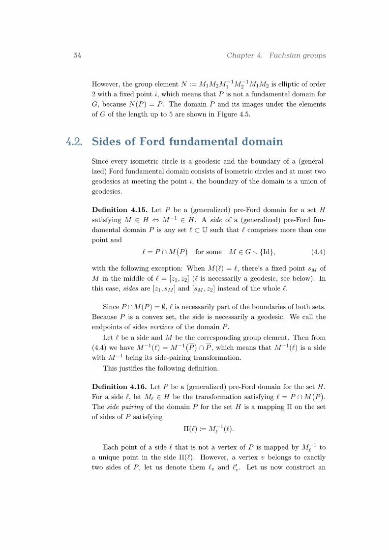
4.2. Sides of Ford fundamental domainSince every isometric circle is a geodesic and the boundary of a (general-

ized) Ford fundamental domain consists of isometric circles and at most two

geodesics at meeting the point i, the boundary of the domain is a union of

geodesics.

Definition 4.15. Let P be a (generalized) pre-Ford domain for a set H

satisfying M ∈ H ⇔ M−1 ∈ H. A side of a (generalized) pre-Ford fun-

damental domain P is any set ` ⊂ U such that ` comprises more than one

point and

` = P ∩M(P)

for some M ∈ Gr {Id}, (4.4)

with the following exception: When M(`) = `, there’s a fixed point sM of

M in the middle of ` = [z1, z2] (` is necessarily a geodesic, see below). In

this case, sides are [z1, sM ] and [sM , z2] instead of the whole `.

Since P ∩M(P ) = ∅, ` is necessarily part of the boundaries of both sets.

Because P is a convex set, the side is necessarily a geodesic. We call the

endpoints of sides vertices of the domain P .

Let ` be a side and M be the corresponding group element. Then from

(4.4) we have M−1(`) = M−1(P)∩ P , which means that M−1(`) is a side

with M−1 being its side-pairing transformation.

This justifies the following definition.

Definition 4.16. Let P be a (generalized) pre-Ford domain for the set H.

For a side `, let M` ∈ H be the transformation satisfying ` = P ∩M(P).

The side pairing of the domain P for the set H is a mapping Π on the set

of sides of P satisfying

Π(`) := M−1` (`).

Each point of a side ` that is not a vertex of P is mapped by M−1` to

a unique point in the side Π(`). However, a vertex v belongs to exactly

two sides of P , let us denote them `v and `′v. Let us now construct an

4.2. Sides of Ford fundamental domain 35

Figure 4.6.Side pairings of the different generalized Ford funda-mental domains for the modular group—the black linecorresponds to the transformation z 7→ −1/z, the redline to z 7→ z + 1 and the green line to z 7→ (z − 1)/z(top); the corresponding graphs GP on the vertices of

the domains (bottom) (cf. Example 4.17).

i−ζ ζ

∞

iζ

∞

0

iζ

∞

η

1/η−1/η

ζ−ζ i

∞∞

0

iζ

−1/η 1/η

η

i

∞

ζ

un-oriented graph‡ GP = (V,E) with V being the vertices of P and edges

E :={{v,M−1

`v(v)}, {v,M−1

`′v(v)}

∣∣v ∈ V }. (4.5)

The connected components of V are either cycle graphs or simple complete

graphs on two vertices or isolated vertices with loops. This is due to the

fact that each vertex has an edge to only itself (if M`v fixes v), to one vertex

(if M−1`v

(v) = M−1`′v

(v), in which case M−1`v

(v) has edge only to v) or to two

vertices (otherwise).

Example 4.17. A side of a domain need not to be a side in the common

sense. In Figure 4.6, we can see that one geodesic comprises more sides

‡Un-oriented graph G is a pair of sets (V, E). The set V is arbitrary set and its elementsare called vertices. The set E is a subset of

`V2

´∪

`V1

´, where

`Vs

´is a set of subsets of

V of the size s; the elements of E are called edges. For e ∈ E, if we have #e = 2 thene = {v, v′} is an edge between vertices v, v′ ∈ V ; if we have #e = 1 then e = {v} is aloop on a vertex v. The set E can be interpreted as a relation “having common edge” onthe set V —let us denote the symmetric, reflexive and transitive closure of this relation ∼.Then the connected component of V is a graph with V ′ ⊆ V being an equivalence class of

∼ and E′ = E ∩“`V ′

2

´∪

`V ′

1

´”. A graph (V, E) is a cycle, we write V = (v0, v1, . . . vr−1),

if E =˘{vk−1, vk}

˛k ∈ {1, . . . , r− 1}

¯∪

˘{v0, v1}

¯. A graph (V, E) is a simple complete

graph if E =`V2

´.


Figure 4.7. To the proof of Theorem 4.18, to illustrate the ‘+’ sign inthe sum of angles: the hyperbolic case in the left and theelliptic case in the right; the parabolic case is analogous

to the elliptic one.

(two in the figure). The figure shows side-pairings for the three fundamental

domains of the modular group, as they are depicted in Figures 4.1 and 4.3.

Below each figure, the corresponging graphs GP are drawn.

Theorem 4.18. Let P be a (generalized) pre-Ford domain for a set of

transformations H. Let C = (v0, v2, . . . vr−1), r ≥ 2, be a cycle of a graph

GP given by (4.5). For k ∈ {0, . . . r − 1}, let Mk ∈ G be the transformation

mapping vk−1 to vk and let αk be the angle between the sides that meet at

vk where we consider the indices modulo r, i.e. v−1 = vr−1 etc.

Denote θ :=∑r−1

j=0 αj and N := Mr−1Mr−2 · · ·M1M0. Then:

(1) N is identity if and only if θ ∈ 2πZ;

(2) N is elliptic with rotN = θ if and only if θ /∈ 2πZ.

Proof. Let `j be the side of P such that M−1j (`j) is a side as well from which

it is clear that the sides meeting at vj are exactly `j and `′j := M−1j+1(`j+1).

The angle between `0 and `′0 is α0.

From the conformity of Möbius transformations we know that the angle

between M0(`0) and M0(`′0) = `1 is α0 as well. The angle between `1 and

`′1 is α1, hence the angle between M0(`0) and `1 is α0 + α1.

Similarly the angle between M1(M0(`0)) and `2 is α0 +α1 +α2. After r

steps we get that the angle betweenMr−1(Mr−2(· · · (M1(M0(`0))))) = N(`0)and `r = `0 is α0 + α1 + · · ·+ αr−1 = θ.

It remains to explain why the angle αk is always added to the sum and

never subtracted. For a hyperbolic transformation Mk, consider the triangle

with vertices sMk(one of its fixed points), and the vertices of `k. Since the


Figure 4.8.An example of a domain with 6 sides and a cycle in thegraph GP of the length 4 (left) and the whole graph GP

(right) (cf. Theorem 4.18).

transformation is orientation-preserving, i.e. it preserves orientation of any

hyperbolic triangles, the side `k is mapped as depicted in Figure 4.7. For

a parabolic or elliptic transformation, consider the vertices of `j and the

fixed point sMk. Since the transformation keeps the hyperbolic distance

unaltered, it preserves the order of these points on the geodesic I(M−1k ), as

depicted in Figure 4.7.

Transformation N fixes the point v0. If θ is a multiple of 2π, N is an

orientation-preserving Möbius transformation that fixes every point on `0

which means that it is the identity. Otherwise it is an elliptic transformation

with θ being its angle of rotation. Q.E.D.

For an illustrative example, see Figure 4.8, where the situation is shown

for a Ford fundamental domain consisting of 6 sides, with a cycle in the

graph GP of the length 4.

The theorem, in many cases, instantly shows the existence of elliptic

element in a group. For instance, the graph GP for the domain in Figure 4.5

(cf. Remark 4.14) is a cycle, all the angles are equal to π/3. This gives that

for each vertex of the domain, there exist an elliptic transformation that

fixes it and has the angle of rotation equal to 2π/3, these group elements

are M1M2M−11 M−1

2 and its conjugates. Beardon [Bea95] does not discuss

the necessity of existence of the elliptic transformations in a Fuchsian group

with a bounded fundamental domain. We state the following conjecture,

whose justification is explained below in Example 4.21.


Conjecture 4.19. There exist a Fuchsian group G with a bounded funda-

mental domain, such that G contains no elliptic transformations.

We will use the following statement from [Kůr09a].

Proposition 4.20. Let 2m, 2n be positive integers such that 1/m+ 1/n < 1.

Put φ := π/n, ψ := π/m and q :=(

1 +√

1− sin2 φ/2cos2 ψ/2

)/(1 −

√1− sin2 φ/2

cos2 ψ/2

).

Let us define the following transformations:

• F0 : z 7→ z/q, hence F0 : z 7→ (q+1)z−i(q−1)i(q−1)z+(q+1) ;

• R : z 7→ eiφz (rotation around 0 by the angle φ in the disc model), i.e.

R : z 7→ z cos φ/2+sin φ/2−z sin φ/2+cos φ/2 ;

• Fk : z 7→ RkF0R−k(z).

Then the set P = U r⋃2nk=0 V (Fk) is a regular 2n-gon whose inner angles

are equal to ψ.

Proof. We first show that q ∈ R and q > 1—for this, see the following

where each inequality implies the next one:

0 < 1/m + 1/n < 1;

cos(π/2m + π/2n) > 0 and cos(π/2m− π/2n) > 0;

2 cos(π/2m + π/2n) cos(π/2m− π/2n) > 0;

cos π/m + cos π/n > 0;

2 cos2 π/2m + 2 cos2 π/2n− 2 > 0;

cos2 π/2m > sin2 π/2m;√1− sin2 φ/2

cos2 ψ/2> 0;

q > 1.

Since R2n = Id, we immediately see that the the set P satisfies a 2nrotational symmetry in the disc model. The value of inner angles can be

computed using Proposition 3.11. For the simplicity, let us measure the

angle between I(F0) and I(F1). Using (3.3), we see that

c0 = iq + 1q − 1

and c1 = c0eiφ. (4.6)

Denote c = |c0| = |c1|. Then |c0 − c1| = 2c sin φ/2 and

−1 +c2

c2 − 1sin2 φ/2 = −2c2 − 4c2 sin2 φ/2− 2

2(c2 − 1)Prop. 3.6======= cosψ = cos2 ψ/2− 1.


Figure 4.9.The pre-Ford domain P from Example 4.21 in blue andthe cycles of graph GP in green and yellow. The inner

angles are all equal to 2π/5.

Let us denote Φ = sin2 φ/2 and Ψ = cos2 ψ/2. Then we can express 1/c in

the terms of Φ,Ψ:

−1 +c2

c2 − 1Φ = Ψ− 1;

c2

c2 − 1= Ψ/Φ;

c2(1−Ψ/Φ) = −Ψ/Φ;

1/c2 = 1− Φ/Ψ.

From (4.6) we see that qc− c = q + 1 and

q =c+ 1c− 1

=1 + 1/c1− 1/c

=1 +

√1− Φ/Ψ

1−√

1− Φ/Ψ. Q.E.D.

Example 4.21. Let us apply the previous proposition to the case n = 5and m = 2.5 and take the group G := 〈F0, F1, . . . F4〉.

As we already said, proving that a group is Fuchsian is generally very

difficult. Suppose now that G is Fuchsian and a pre-Ford domain for the

set of transformations {F0, . . . , F4, F−10 , . . . , F−1

4 } is its Ford fundamental

domain.


This domain is, according to the previous proposition, a regular hy-

perbolic 10-gon with the angles at its vertices all equal to 2π/5 and it is

bounded. This domain embodies a side-pairing given by the generators Fk.

The graph GP comprises two cycles of the length 5. (In Figure 4.9, the sides

of P are depicted in blue, its vertices in black, and the graph GP in green

and yellow.)

For Theorem 4.18, we have all αk equal to 2π/5 and r = 5, hence

θ = 2π. This means that the transformations satisfy F0F2F4F−11 F−1

3 =F0F

−13 F−1

1 F4F2 = Id, which is obviously true for all the conjugates of these

two as well.

Under the assumption that P is a fundamental domain, we get that

the group contains no elliptic transformations—if there existed an elliptic

M ∈ G, its fixed point would have to be a vertex of an image of P , and by

conjugation there exists another elliptic M1 ∈ G with the fixed point being a

vertex of P itself, let us denote it v. Then M1(P ) meets the neighborhood of

v, but the neighborhood of v is tessellated by images of P under hyperbolic

transformations, contradiction. This led us to state Conjecture 4.19.

CHAPTER 5

Rational groups with abounded fundamental

domain

Julius Wilhelm Richard Dedekind (1831–1916)German mathematician, worked in algebra and the foundations of the

real numbers, discovered the tessellation by the modular group.

42 Chapter 5. Rational groups with a bounded fundamental domain

Table 5.1. The significant values of the trace of a Möbius transfor-mation.

tr2M rotM = 2 arccos√

tr2M2 order of M

0 π 21 2π/3 32 π/2 43 π/3 6

Our concern is to study rational groups, i.e. groups of transformationswith matrices in PGL+(2,Z), which comprises matrices with integer coeffi-cients and a positive determinant. Let us recall that we identify the matricesA and λA, which means that

(a bc d

)−1 = 1det A

(d −b−c a

)=(d −b−c a

); for the same

reason we speak about “rational groups” and consider the matrices to haveinteger coefficients.

In Examples 4.2 and 4.5 we show that there exist rational Fuchsiangroups, but in both cases, their fundamental domain is unbounded.

We have not found any example of a rational Fuchsian group withbounded fundamental domain, so we stated the following conjecture.

Conjecture 5.1. There is no rational Fuchsian group with a bounded fun-damental domain.

However, the proof of this conjecture seems to be unreachable. Eventhough, we try to investigate some cases.

5.1. Groups with elliptic elementsSuppose first that the group G contains elliptic elements. Since we considerFuchsian groups, the angle of rotation of any elliptic M ∈ G satisfy rotM ∈πQ; or in the case rotM /∈ πQ, the powers of M accumulate in M(2,R).This puts a restriction on the values of the trace tr2M .

Proposition 5.2. Let G be a rational Fuchsian group and M ∈ G be an

elliptic transformation. Then

tr2M ∈ {0, 1, 2, 3}.

Proof. From Proposition 3.4 we know that tr2M = 4 cos2 rotM2 . Any angle

θ satisfies 2 cos2 θ = 1 + cos 2θ. Hence tr2M = 2(1 + cos rotM). BecauseAM has rational elements, tr2M ∈ Q, which follows to cos rotM ∈ Q.

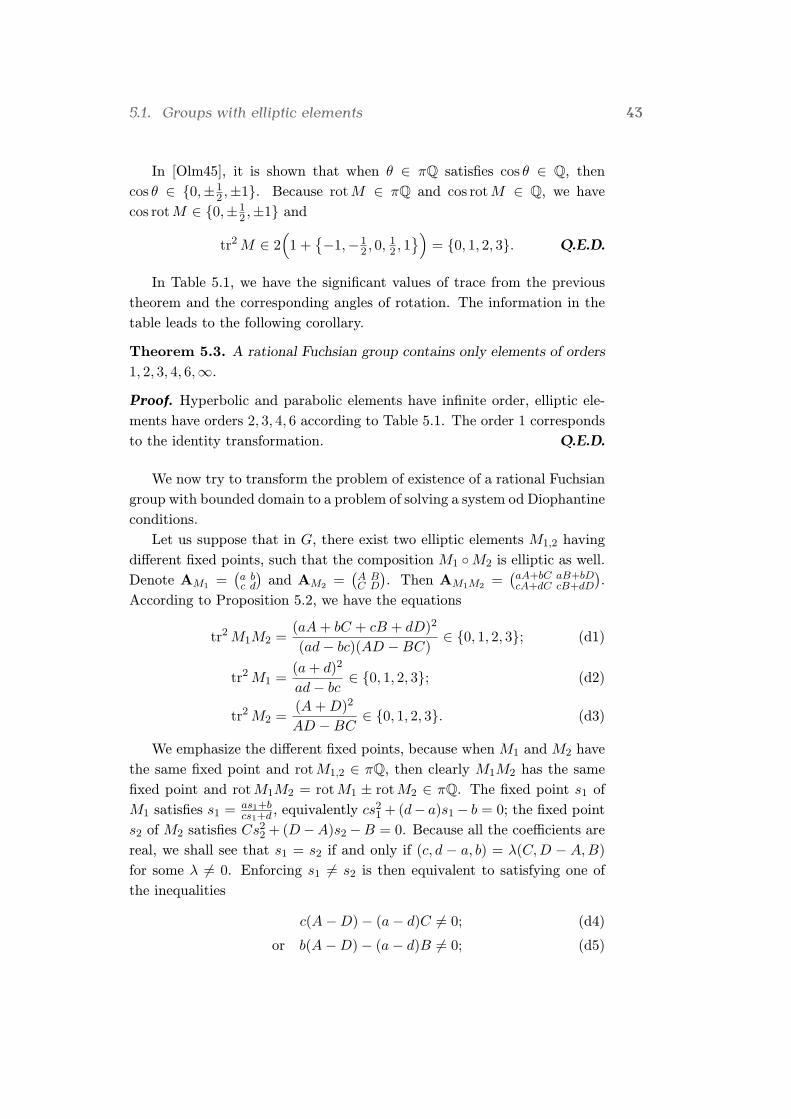
5.1. Groups with elliptic elements 43

In [Olm45], it is shown that when θ ∈ πQ satisfies cos θ ∈ Q, then

cos θ ∈ {0,±12 ,±1}. Because rotM ∈ πQ and cos rotM ∈ Q, we have

cos rotM ∈ {0,±12 ,±1} and

tr2M ∈ 2(

1 +{−1,−1

2 , 0,12 , 1})

= {0, 1, 2, 3}. Q.E.D.

In Table 5.1, we have the significant values of trace from the previous

theorem and the corresponding angles of rotation. The information in thetable leads to the following corollary.

Theorem 5.3. A rational Fuchsian group contains only elements of orders

1, 2, 3, 4, 6,∞.

Proof. Hyperbolic and parabolic elements have infinite order, elliptic ele-

ments have orders 2, 3, 4, 6 according to Table 5.1. The order 1 corresponds

to the identity transformation. Q.E.D.

We now try to transform the problem of existence of a rational Fuchsian

group with bounded domain to a problem of solving a system od Diophantine

conditions.

Let us suppose that in G, there exist two elliptic elements M1,2 having

different fixed points, such that the composition M1 ◦M2 is elliptic as well.

Denote AM1 =(a bc d

)and AM2 =

(A BC D

). Then AM1M2 =

(aA+bC aB+bDcA+dC cB+dD

).

According to Proposition 5.2, we have the equations

tr2M1M2 =(aA+ bC + cB + dD)2

(ad− bc)(AD −BC)∈ {0, 1, 2, 3}; (d1)

tr2M1 =(a+ d)2

ad− bc∈ {0, 1, 2, 3}; (d2)

tr2M2 =(A+D)2

AD −BC∈ {0, 1, 2, 3}. (d3)

We emphasize the different fixed points, because when M1 and M2 have

the same fixed point and rotM1,2 ∈ πQ, then clearly M1M2 has the same

fixed point and rotM1M2 = rotM1 ± rotM2 ∈ πQ. The fixed point s1 of

M1 satisfies s1 = as1+bcs1+d , equivalently cs2

1 + (d− a)s1− b = 0; the fixed point

s2 of M2 satisfies Cs22 + (D−A)s2 −B = 0. Because all the coefficients are

real, we shall see that s1 = s2 if and only if (c, d − a, b) = λ(C,D − A,B)for some λ 6= 0. Enforcing s1 6= s2 is then equivalent to satisfying one of

the inequalities

c(A−D)− (a− d)C 6= 0; (d4)

or b(A−D)− (a− d)B 6= 0; (d5)


let us denote the last two left-side terms ωc and ωb, respectively.

All these considerations can be summarized in the following way.

Theorem 5.4. Suppose that the system of conditions (d1)–(d5) has no

integer solutions. Then there exist no rational Fuchsian group G containing

elliptic transformation M1,2 with different fixed points such that M1M2 is

elliptic.

Unfortunately, this theorem gives only a partial results, in 2 senses:

(1) we do not know whether the system has integer solutions;

(2) we do not know whether elliptic transformations have to be contained

in a Fuchsian group with a bounded fundamental domain;

(3) we do not know whether when the group contains elliptic transfor-

mations, it contains an elliptic composition of elliptic transformations

with different fixed points.

These three questions are essential for the Conjecture 5.1. The previous

theorem would then answer the conjecture for a broad family of Fuchsian

groups, but it would not answer it completely.

Using a computer simulation, we have shown the following.

Claim 5.5. The system of conditions (d1)–(d5) has no integer solution with

a, b, c, d, A,B,C,D ∈ {−100,−99 . . . , 99, 100}.

The description of the program can be found in Section 5.2. To make

the program run significantly faster, we use following several symmetries of

the conditions:

Lemma 5.6. Let Sol be the set 8-tuplets (a, b, c, d, A,B,C,D) ∈ Z8 of the

solutions of the system (d1)–(d5). Then

v(1) := (a, b, c, d, A,B,C,D) ∈ Sol

⇐⇒ v(2) := (A,B,C,D, a, b, c, d) ∈ Sol

⇐⇒ v(3) := (a, c, b, d, A,C,B,D) ∈ Sol

⇐⇒ v(4) := (d, b, c, a,D,B,C,A) ∈ Sol

⇐⇒ v(5) := (−a, b, c,−d,−A,B,C,−D) ∈ Sol

⇐⇒ v(6) := (a,−b,−c, d,A,−B,−C,D) ∈ Sol

5.1. Groups with elliptic elements 45

Proof. Let us denote fi(a, b, c, d, A,B,C,D) the formula in the condition

(di), for i = 1, . . . , 5. Then clearly

f1(v(1)) = f1(v(2)) = f1(v(3)) = f1(v(4)) = f1(v(5)) = f1(v(6)),

f2(v(1)) = f3(v(2)) = f2(v(3)) = f2(v(4)) = f2(v(5)) = f2(v(6)),

f3(v(1)) = f2(v(2)) = f3(v(3)) = f3(v(4)) = f3(v(6)) = f3(v(6)),

f4(v(1)) = −f4(v(2)) = f5(v(3)) = −f4(v(4)) = −f4(v(5)) = −f4(v(6)),

f5(v(1)) = −f5(v(2)) = f4(v(3)) = −f5(v(4)) = −f5(v(5)) = −f5(v(6)),

which is satisfactory for the equivalence of the solutions of the system.

Q.E.D.

Example 5.7. We now show a few examples of “partial solutions”—when

we omit some of the conditions, we get a solvable Diophantine system.

• Let AM1 =(

6 −37 −3

)and AM2 =

(5 −48 −5

). Then both M1 and M2 are

elliptic and have different fixed points, because c(A−D)− (a−d)C =2 6= 0 and b(A−D)− (a−d)B = 6 6= 0. The traces satisfy tr2M1 = 0,

tr2M2 = 3 and tr2M1M2 = 73 , hence M1M2 is elliptic with infinite

order.

This means that if we modify (d1) to tr2M1M2 ∈ [0, 4), i.e. M1M2 is

elliptic but with a general value of trace, we find a solution.

• Let AM1 =(

1 10−5 −1

)and AM2 =

(0 −11 1


elliptic and have different fixed points, because c(A−D)−(a−d)C = 3and b(A − D) − (a − d)B = −8. The traces satisfy tr2M1 = 0,

tr2M2 = 1 and tr2M1M2 = 4, hence M1M2 is parabolic and not

elliptic.

This means that if we modify (d1) to tr2M1M2 ∈ N0, i.e. M1M2 is

generally not elliptic but has an integer trace, we find a solution.

• Let AM1 =(

1 10−5 −1

)and AM2 =

(0 −11 1


elliptic and have the same fixed point, because c(A−D)− (a− d)C =b(A −D) − (a − d)B = 0. The traces satisfy tr2M1 = 3, tr2M2 = 1and tr2M1M2 = 3, hence M1M2 is elliptic and has the finite order.

This means that if we omit (d4), (d5), i.e. we allow M1 and M2 to

have the same fixed point, we find a solution.

These examples are summarized in Table 5.2, with two additional ones.


Tabl

e5.

2.Th

eex

ampl

esofM

1,M

2su

chth

atth

eel

emen

tsof

thei

rm

atri

ces

AM

1an

dAM

2so

lve

som

eof

the

cond

ition

s.W

ede

noteωc: =c(A−D

)−

(a−d)C

and

ωb: =b(A−D

)−

(a−d)B

.

Equ

atio

n:

(d1)

(d2)

(d3)

(d4)

(d5)

Qu

anti

ty:

(a,b,c,d

)(A,B,C,D

)tr

2M

1tr

2M

2tr

2M

1M

2ωc

ωb

Con

dit

ion

:∈

Z4∈

Z4∈{0,...,3}∈{0,...,3}∈{0,...,3}6=

06=

0

(6,−

3,7,−

3)(5,−

4,8,−

5)0

37/

32

6

(1,1

0,−

5,−

1)(0,−

1,1,

1)0

14

3−

8

(4,−

1,4,

2)(0,1,−

4,2)

31

30

0

(11,−

7,13,1

9)(−

4,−

7,13,4

)0

31

00

(−1,

5,−

1,3)

(2,−

5,1,−

2)2

20

00

5.2. Program for the Diophantine system 47

5.2.Program for finding solutions of theDiophantine system

In Claim 5.5, we state that the system of Diophantine conditions (d1)–(d5)

has no integer solutions with all unknowns in modulus less than or equal to

100.

To show this statement, we used a computer program written in the

programming language C++. The program is not long, which allows us to

explain its principles in detail.

Headers for text output handling.

1 #include<iostream>

2 using namespace std;

LL is a type we use to store integers. The maximum value of number in LL

is (at our machine) over 9 · 1018, as we checked by LONG MAX in the module

<climits>.

3 typedef long int LL;

We use the Euclid algorithm to compute the greatest common divisor of two

numbers. We have to deal with the input a = b = 0, for which the value

of gcd is undefined in mathematics; we set the result to 0 in this case, since

in the end, we compute gcd(a, b, c, d) and if all of them are 0, the matrix is

singular and we exclude it no matter the value of gcd.

4 LL gcd(LL a, LL b){

5 if(a<0) a=-a;

6 if(b<0) b=-b;

7 if((a==0)&&(b==0)) return 0;

8 if(a==0) return b;

9 if(b==0) return a;

10 LL c=a%b;

11 while(c!=0){

12 a=b;

13 b=c;

14 c=a%b;

15 }

16 return b;

17 }

The largest numbers we manipulate are squared traces of products of ma-

trices, i.e. numbers of the form (XX + XX + XX + XX)2 where X stands for a

coefficient in the matrix. This is in modulus smaller than 16 · M4, where M


is the upper bound for the coefficients. We restrict ourselves to M ≤ 2 · 104,

which gives 16 · M4 < 3 · 1018 < LONG MAX.

The maximal choice M = 20 000 would make our simulation run for ages.

Thus we bound the coefficients by much smaller M = 100.

18 const LL M=100;

The main program.

19 int main(){

We need several integer variables: for the matrices’ coefficients, determi-

nants, to store some greatest common divisor (see later) and traces of the

matrices. We work with matrices M1 = (a bc d) and M2 = (A B

C D).20 LL a,b,c,d,A,B,C,D;

21 LL xdet,xDET;

22 LL xgcd;

23 LL t,T,Tt;

The main part of the program. It comprises 8 nested for-loops, each for one

coefficient of the matrices M1, M2. At various places we exclude such com-

binations of coefficients that cannot lead to a new solution of the equations.

24 for(a=-M; a<=M; a++){

Printing verbose information to enable checking the progress.

25 cout << "*** a = " << a << " ***" << endl;

26 for(b=-M; b<=M; b++){

27 xgcd=gcd(a,b);

Lemma 5.6, relation v(1) ∈ Sol⇔ v(3) ∈ Sol, gives that if there is a solution

with b ≤ c, then there is a solution with c ≤ b as well. Therefore we can

restrict the simulation to c ≤ b.

28 for(c=-M; c<=b; c++){

29 xgcd=gcd(xgcd,c);


with a ≤ d, then there is a solution with d ≤ a as well.

30 for(d=-M; d<=a; d++){

In the four outer for-loops, we compute the number xgcd = gcd(a, b, c, d).The 4-tuplets such that xgcd > 1 cannot bring a new solution since for such

solution, there must be one for a 4-tuplet (a/xgcd, b/xgcd, c/xgcd, d/xgcd)as well.

31 if(gcd(xgcd,d)!=1) continue;

The matrix M1 cannot have negative or zero determinant.

32 xdet=a*d-b*c;

33 if(xdet<=0) continue;

Trace squared of the matrix M1.

5.2. Program for the Diophantine system 49

34 t=(a+d)*(a+d);

The trace square of the transformation is tr2M1detM1

. We exclude such matrices

that tr2M1detM1

≥ 4, which can be rewritten as tr2M1 ≥ 4 detM1 to avoid divi-

sions.

35 if(t>=4*xdet) continue;

The trace has to be an integer, which means that the division detM1÷tr2M1

cannot give a non-zero residue.

36 if((t%xdet)!=0) continue;

Lemma 5.6, relation v(1) ∈ Sol⇔ v(5), v(6) ∈ Sol, allows us to omit negative

values of A and B, since the existence of a solution with negative A, B enforces

the existence of a solution with non-negative values.

37 for(A=0; A<=M; A++){

38 for(B=0; B<=M; B++){

39 for(C=-M; C<=M; C++){


with d ≤ D, then there is a solution with D ≤ d as well.

40 for(D=-M; D<=d; D++){

Now follows conditions on detM2 and tr2M2, analogous to those for M1.

41 xDET=A*D-B*C;

42 if(xDET<=0) continue;

43 T=(A+D)*(A+D);

44 if(T>=4*xDET) continue;

45 if((T%xDET)!=0) continue;

We compute the trace squared of a matrix M1M2 and perform similar re-

strictions as on M1 and M2.

46 Tt=a*A+b*C+c*B+d*D;

47 Tt=Tt*Tt; // trace squared of M1*M2

48 if(Tt>=4*xdet*xDET) continue;

49 if((Tt%(xdet*xDET))!=0) continue;

Finally, we forbid M1 and M2 to have the same fixed point.

50 if(

51 (c*(A-D)-(a-d)*C==0)

52 &&

53 (b*(A-D)-(a-d)*B==0)

54 ) continue;

When we get to this point, we get a solution of the system which we print.

55 cout << "solution: a,b,c,d,A,B,C,D = "

56 << a << "," << b << ","

57 << c << "," << d << ","


58 << A << "," << B << ","

59 << C << "," << D << ","

60 << endl;

Terminate the for-loops and exit the program.

61 }}}}}}}}

62 return 0;

63 }

CHAPTER 6

Conclusions

52 Chapter 6. Conclusions

This thesis studies some aspects of Fuchsian groups and aims on the groups

of rational transformations. We have not been able to provide a definite an-

swer to the question of existence of such groups. In Chapter 5, we conjecture

that no such groups exist, and we support this conjecture by a computer

experiment that is described in Section 5.2. Very important condition is

given in Theorem 5.3.

Beside the discussion on rational groups, we proved several interesting

results:

• Theorem 4.9, which generalizes the result in [For25];

• Theorem 4.12, which provides a large family of Fuchsian groups that

contain no elliptic transformations and their fundamental domain is

unbounded;

• Theorem 4.18, which allows to compute the angle of rotation of elliptic

transformations fixing the vertices of (generalized) Ford fundamental

domains and pre-Ford domains.

6.1. Open problemsThe problem of existence of a rational Fuchsian group with bounded funda-

mental domain remains open. As well, more investigations in the theory of

Möbius number systems can be done. Especially, only orientation-preserving

Möbius transformations have been considered in these systems. If we add

the orientation-reversing Möbius transformations, i.e. such Ma,b,c,d that

ad−bc < 0, we get the general Möbius group GM(2,R). The group M(2,R)is a subgroup of GM(2,R) of the index 2. Expanding to general the Möbius

group would allow to use the knowledge on Möbius number systems to the

simple continued fraction, and to the radix representations with the negative

base, such as the Ito-Sadahiro numeration [IS09].

Bibliography

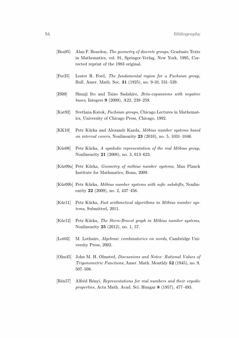
54 Bibliography

[Bea95] Alan F. Beardon, The geometry of discrete groups, Graduate Texts

in Mathematics, vol. 91, Springer-Verlag, New York, 1995, Cor-

rected reprint of the 1983 original.

[For25] Lester R. Ford, The fundamental region for a Fuchsian group,

Bull. Amer. Math. Soc. 31 (1925), no. 9-10, 531–539.

[IS09] Shunji Ito and Taizo Sadahiro, Beta-expansions with negative

bases, Integers 9 (2009), A22, 239–259.

[Kat92] Svetlana Katok, Fuchsian groups, Chicago Lectures in Mathemat-

ics, University of Chicago Press, Chicago, 1992.

[KK10] Petr Kůrka and Alexandr Kazda, Möbius number systems based

on interval covers, Nonlinearity 23 (2010), no. 5, 1031–1046.

[Kůr08] Petr Kůrka, A symbolic representation of the real Möbius group,

Nonlinearity 21 (2008), no. 3, 613–623.

[Kůr09a] Petr Kůrka, Geometry of möbius number systems, Max Planck

Institute for Mathmatics, Bonn, 2009.

[Kůr09b] Petr Kůrka, Möbius number systems with sofic subshifts, Nonlin-

earity 22 (2009), no. 2, 437–456.

[Kůr11] Petr Kůrka, Fast arithmetical algorithms in Möbius number sys-

tems, Submitted, 2011.

[Kůr12] Petr Kůrka, The Stern-Brocot graph in Möbius number systems,

Nonlinearity 25 (2012), no. 1, 57.

[Lot02] M. Lothaire, Algebraic combinatorics on words, Cambridge Uni-

versity Press, 2002.

[Olm45] John M. H. Olmsted, Discussions and Notes: Rational Values of

Trigonometric Functions, Amer. Math. Monthly 52 (1945), no. 9,

507–508.

[Rén57] Alfréd Rényi, Representations for real numbers and their ergodic

properties, Acta Math. Acad. Sci. Hungar 8 (1957), 477–493.

55

[wiki1] Wikipedia, Parallel postulate,

http://en.wikipedia.org/wiki/Parallel_postulate,

2011, [online; accessed 15 Nov 2011].

[wiki2] Wikipedia, August Ferdinand Möbius,

http://en.wikipedia.org/wiki/August_Ferdinand_Mobius,

2012, [online; accessed 15 Mar 2012].

[wiki3] Wikipedia, Henri Poincaré,

http://en.wikipedia.org/wiki/Henri_Poincare,


[wiki4] Wikipedia, Lazarus Fuchs,

http://en.wikipedia.org/wiki/Lazarus_Fuchs,


[wiki5] Wikipedia, Modular group,

http://en.wikipedia.org/wiki/Modular_group,


[wiki6] Wikipedia, Polymath,

http://en.wikipedia.org/wiki/Polymath,


[wiki7] Wikipedia, Richard Dedekind,

http://en.wikipedia.org/wiki/Richard_Dedekind,


[www1] Lieven Le Bruyn, Dedekind or Klein ?,

http://www.neverendingbooks.org/index.php/

dedekind-or-klein.html,


Index of Notations

58 Index of Notations

Symbol Description

N natural numbers, N := {0, 1, 2, 3, · · · }Z integer numbers, Z := {· · · ,−3,−2,−1, 0, 1, 2, 3, · · · }Q rational numbersR real numbersC complex numbersarg z argument of a complex number z, z = |z| ei arg z

<z,=z real and imaginary component of a complex number,z = <z + i=z

z complex conjugate of z ∈ C, z = <z − i=z#X number of elements of the set X

R extended real line, R := R ∪ {∞}C extended complex plane, C := C ∪ {∞}U upper complex half-plane, U := {z ∈ C | =z > 0}∂U boundary of U, synonym for RD unit complex disc, D := {z ∈ C | |z| < 1}∂D boundary of D, ∂D := {z ∈ C | |z| = 1}

[z1, z2] geodesic between points z1 and z2

ρ(z1, z2) hyperbolic distance of two points, the hyperboliclength of [z1, z2].

Q topological closure of Q in UQ topological closure of Q in U ∪ ∂U

GL+(2,R) group of 2× 2 real matrices with strictly positivedeterminant

PGL+(2,R) group GL+(2,R)/∼, where A ∼ B iff(∃λ ∈ R, λ 6= 0)(B = λA)

PSL(2,Z) group of 2× 2 integer matrices with determinant 1,factorized by {I,−I}

M(2,R) group of all orientation-preserving real Möbiustransformations

M(2,Z) group of all orientation-preserving real Möbiustransformations with integer coefficients

GM(2,R) group of all real Möbius transformations(a bc d

)typical notation of coefficients of a matrix of a Möbius

transformation in the half-plane model(α ββ α

)typical notation of coefficients of a matrix of a Möbius

transformation in the disc modelM• circle derivative of MI(M) isometric circle of MV (M) expansion area of MXF convergence space for the system F

59

Symbol Description

〈g1, . . . , gm〉 group generated by the elements g1, . . . , gmleng1,g2,...,gk(h) length of h ∈ 〈g1, . . . , gm〉

A alphabet, in general any finite set with #A ≥ 2A∗ the set of finite words over the alphabet Au∗ the set of words of the form uk for k ∈ NAN the set of right infinite words over the alphabet AuN the ultimately periodic infinite word uN = uuu · · ·ΣX subshift of finite type with forbidden set of factors X

General Index

62 General Index

Aacting discontinuously, 26

alphabet, 8

angle of rotation, 17

Cclosure

hyperbolic, 15

concatenation of words, 8

continued fraction, 10

alternating, 11

cycle, 35

cylinder, 8

Dderivative

circle, 18

domain

generalized pre-Ford, 29

pre-Ford, 28

Eedge

of graph, 35

expansion area, 18

Ffactor, 8

fundamental domain, 26

Ford, 30

generalized Ford, 30

Ggeodesic, 14

graph, 35

simple complete, 35

un-oriented, 35

group

Fuchsian, 26

general Möbius, 52

Möbius, 16

modular, 12, 26

rational, 42

Iisometric circle, 18

isometry, 15

Llanguage, 8

length

of group element, 10

of word, 8

MMöbius iterative system, 9

Möbius number system, 9

redundant, 9

Möbius transformation

elliptic, 16

hyperbolic, 16

in hyperbolic geometry, 15

orientation-reversing, 52

parabolic, 16

rational, 17

real orientation-preserving, 9

map

conformal, 14, 15

isometry, 15

metric

hyperbolic, 14

63

Pprefix, 8

RRényi positional system, 10

reflection

in circle, 21

in line, 21

Sset

clopen, 8

SFT, 9

shift

full, 9

shift map, 8

side

of pre-Ford domain, 34

side pairing, 34

space

convergence, 9

straight line

hyperbolic, 14

subshift, 8

of finite type, 9

substitution, 8

suffix, 8

infinite, 8

symbolic representation, 9

Ttail, 8

trace

of Möbius transformation, 17

of matrix, 17

Uunit disc, 14

upper half plane, 14

Vvertex

of fundamental domain, 34

of graph, 35

Wword, 8

forbidden, 9

This thesis was typeset in the LATEX 2ε typesettingsystem, with report class and additional packages

amsfonts, amsmath, amssymb, amsthm, babel, bm, booktabs,fancyhdr, floatrow, fontenc, geometry, graphicx,inputenc, ltablex, makeidx, mathtools, nicefrac,

relsize, rotating, tikz, titlesec, tocloft, url, xcolor,as well as with various author’s customizations. The

figures were drawn by hand or using the Maplesoftware. The typefaces used are Computer Modern

and Antykwa Toruńska. The source files of the thesis aswell as all the figures can be found on the website

http://kmlinux.fjfi.cvut.cz/~hejdato1

Colophon

This work was supported by the Grant Agency of theCzech Technical University in Prague, grant No.

SGS11/162/OHK4/3T/14and Czech science foundation grant

GAČR 201/09/0584

Acknowledgements

Date post:	15-Feb-2019
Category:	Documents
Upload:	doquynh
View:	215 times
Download:	0 times

Moebiovské systémy numerace s diskrétními grupami Moebius...

Documents